Chapter 5 Code#
We will use the following imports.
import numpy as np
import matplotlib.pyplot as plt
from numba import jit
The Optimal Savings Problem#
First we set parameters and construct the state and action spaces.
beta, rho = 0.5, 0.9
z_bar, s_bar = 10, 5

S = np.arange(z_bar + s_bar + 1)    # State space = 0,...,z_bar + s_bar
Z = np.arange(z_bar + 1)            # Shock space = 0,...,z_bar
Next we write down the primitives of the problem, such as the utility function.
def U(c):
    "Utility function."
    return c**beta

def phi(z):
    "Probability mass function, uniform distribution."
    return 1.0 / len(Z) if 0 <= z <= z_bar else 0

def Gamma(x):
    "The correspondence of feasible actions."
    return range(min(x, s_bar) + 1)
Value Function Iteration#
To implement VFI, we first construct the Bellman operator \(T\).
def T(v):
    Tv = np.empty_like(v)
    for x in S:
        # Compute the value of the objective function for each
        # a in Gamma(x) and record highest value.
        running_max = -np.inf
        for a in Gamma(x):
            y = U(x - a) + rho * sum(v[a + z]*phi(z) for z in Z)
            if y > running_max:
                running_max = y
        # Store the maximum reward for this x in Tv
        Tv[x] = running_max
    return Tv
The next function computes a \(w\)-greedy policy.
def get_greedy(w):
    sigma = np.empty_like(w)
    for x in S:
        running_max = -np.inf
        for a in Gamma(x):
            y = U(x - a) + rho * sum(w[a + z]*phi(z) for z in Z)
            # Record the action that gives highest value
            if y > running_max:
                running_max = y
                sigma[x] = a
    return sigma
The following function implements value function iteration, starting with the utility function as the initial condition.
Iteration continues until the sup deviation between iterates is less than
tol.
def compute_value_function(tol=1e-4,
                           max_iter=1000,
                           verbose=True,
                           print_skip=5):

    # Set up loop
    v = [U(x) for x in S]     # Initial condition
    i = 0
    error = tol + 1

    while i < max_iter and error > tol:
        v_new = T(v)
        error = np.max(np.abs(v - v_new))
        i += 1
        if verbose and i % print_skip == 0:
            print(f"Error at iteration {i} is {error}.")
        v = v_new

    if i == max_iter:
        print("Failed to converge!")

    if verbose and i < max_iter:
        print(f"\nConverged in {i} iterations.")

    return v_new
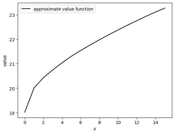
Let’s run the code and plot the result.
v_star = compute_value_function()

fig, ax = plt.subplots()
ax.plot(S, v_star, 'k-', label='approximate value function')
ax.legend()
ax.set_xlabel("$x$")
ax.set_ylabel("value")

#plt.savefig("vfiv.pdf")

plt.show()
Error at iteration 5 is 1.2573668687016468.
Error at iteration 10 is 0.741211643809562.
Error at iteration 15 is 0.4376689170549888.
Error at iteration 20 is 0.2584390462574362.
Error at iteration 25 is 0.15260567184870055.
Error at iteration 30 is 0.09011212316537609.
Error at iteration 35 is 0.05321030760788403.
Error at iteration 40 is 0.0314201545393793.
Error at iteration 45 is 0.018553287053961753.
Error at iteration 50 is 0.010955530472493535.
Error at iteration 55 is 0.0064691311887052905.
Error at iteration 60 is 0.003819957275620567.
Error at iteration 65 is 0.002255646571679648.
Error at iteration 70 is 0.0013319367441120278.
Error at iteration 75 is 0.0007864953280325437.
Error at iteration 80 is 0.00046441762625448746.
Error at iteration 85 is 0.0002742339641272906.
Error at iteration 90 is 0.00016193241347650655.
Error at iteration 95 is 9.561947083724931e-05.

Converged in 95 iterations.
Now we can compute the \(v^*\)-greedy policy, which is approximately optimal.
sigma_star = get_greedy(v_star)

fig, ax = plt.subplots()
ax.plot(S, sigma_star, 'k-', label='optimal policy')
ax.legend()

plt.show()
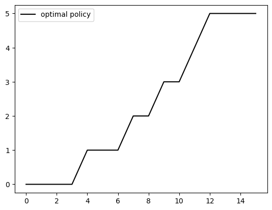
Even though value function iteration only guarantees an approximately optimal policy, since computation of the value function is only up to a certain degree of precision, it turns out that our policy is exactly optimal.
This becomes clear in the next section.
Before that, let’s check that the Markov chain for wealth is globally stable by calculating the Dobrushin coefficient.
Here’s a function to compute the Dobrushin coefficient.
def dobrushin(p):
    running_min = 1
    for x in S:
        for xp in S:
            a = sum((min(p[x,y], p[xp, y]) for y in S))
            if a < running_min:
                running_min = a
    return running_min
Now we construct the stochastic kernel at the optimal policy and check the Dobrushin coefficient.
p_sigma = np.empty((len(S), len(S)))

for x in S:
    for y in S:
        p_sigma[x, y] = phi(y - sigma_star[x])

dobrushin(p_sigma)
0.5454545454545455
The Dobrushin coefficient is positive so global stability holds.
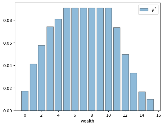
We’ll borrow some earlier code to compute the stationary distribution.
from numpy.linalg import solve

def compute_stationary(p):
    N = p.shape[0]
    I = np.identity(N)
    O = np.ones((N, N))
    A = I - p + O
    return solve(A.T, np.ones((N, 1))).flatten()
Now let’s compute it.
fig, ax = plt.subplots()
psi_star = compute_stationary(p_sigma)

ax.bar(S, psi_star, edgecolor='k', alpha=0.5, label=r'$\psi^*$')
ax.set_xlabel('wealth')
ax.legend()

# plt.savefig("opt_wealth_dist.pdf")

plt.show()
Policy Iteration#
Now we turn to the Howard policy iteration algorithm.
In the finite state setting, this algorithm converges to the exact optimal policy.
To implement the algorithm, we need to be able to evaluate the lifetime reward of any given policy.
The next function does this using the algebraic method suggested in the textbook.
def compute_policy_value(sigma):

    # Construct r_sigma and p_sigma = M_sigma
    n = len(S)
    r_sigma = np.empty(n)
    p_sigma = np.empty((n, n))
    for x in S:
        r_sigma[x] = U(x - sigma[x])
        for y in S:
            p_sigma[x, y] = phi(y - sigma[x])


    # Solve sigma = (I - rho p_sigma)^{-1} r_sigma
    I = np.identity(n)
    sigma = np.linalg.solve(I - rho * p_sigma, r_sigma)
    return sigma
Now we can implement policy iteration.
def policy_iteration(max_iter=1e6, verbose=True):

    sigma = np.zeros(len(S))  # Starting point
    i = 1

    while i < max_iter:
        v_sigma = compute_policy_value(sigma)
        new_sigma = get_greedy(v_sigma)
        if np.all(new_sigma == sigma):
            break
        else:
            sigma = new_sigma
            i += 1

    if i == max_iter:
        print("Failed to converge!")

    if verbose and i < max_iter:
        print(f"\nConverged in {i} iterations.")

    return sigma
Now let’s compute using policy iteration and plot.
sigma_star_pi = policy_iteration()

fig, ax = plt.subplots()
ax.plot(S, sigma_star_pi, 'k-', label='optimal policy via PI')
ax.legend()
ax.set_xlabel("$x$")
ax.set_ylabel("savings")

# plt.savefig("wealth_opt_pol.pdf")

plt.show()
Converged in 4 iterations.
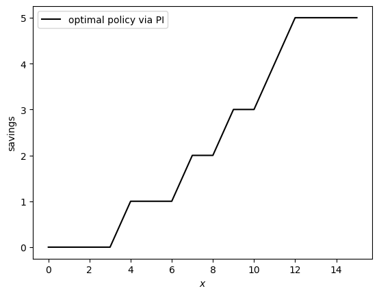
Let’s check that the two ways of computing the optimal policy are equivalent up.
np.all(sigma_star == sigma_star_pi)
True
Success! We have found the optimal policy and both methods of computing lead us to it.
Equilibrium Selection#
Here are the parameter values.
N = 12
u = 2
w = 1
@jit
def reward1(z):
    return (z/N) * u

@jit
def reward2(z):
    return ((N - z)/N) * w

@jit
def B(z):
    if reward1(z) > reward2(z):
        return N
    elif reward1(z) < reward2(z):
        return 0
    else:
        return z

@jit
def update(z, epsilon):
    Vu = np.random.binomial(N - B(z), epsilon)
    Vw = np.random.binomial(B(z), epsilon)
    return B(z) + Vu - Vw
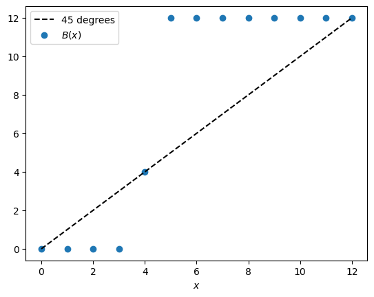
Plot the function \(B\) as a 45 degree diagram.
fig, ax = plt.subplots()
state = np.arange(0, N+1)
ax.plot(state, state, 'k--', label='45 degrees')
ax.scatter(state, [B(x) for x in state], label='$B(x)$')
ax.legend()
ax.set_xlabel('$x$')
# plt.savefig("os_rewards.pdf")
plt.show()
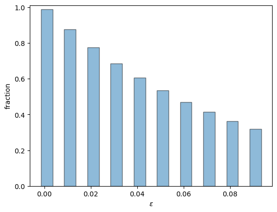
Now we barplot the fraction of time sample paths spend at \(N\) as epsilon varies.
@jit
def compute_time_at_state(s, epsilon, sim_length=1_000_000, x_init=5):
    X = x_init
    counter = 0
    for t in range(sim_length):
        X = update(X, epsilon)
        if X == s:
            counter += 1
    return counter / sim_length

epsilons = np.arange(0.001, 0.1, step=0.01)
sample_frac = np.empty(len(epsilons))
for i, eps in enumerate(epsilons):
    sample_frac[i] = compute_time_at_state(N, eps)

fig, ax = plt.subplots()
ax.bar(epsilons, sample_frac, width=0.005, edgecolor='k', alpha=0.5)
ax.set_ylim(0, 1.01)
ax.set_xlabel('$\\epsilon$')
ax.set_ylabel('fraction')
#plt.savefig("mutation_ess.pdf")
plt.show()