Chapter 11 Code

We begin with some imports

import numpy as np
import matplotlib.pyplot as plt
from numba import njit

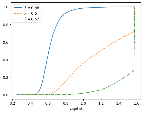
Now we recreate figure 11.3. Our first step is to set the parameters.

alpha = 0.6
Q = 2
R = 1
sigma = 0.1 # variance
mu = - sigma**2 / 2

Next we introduce useful functions.

@njit
def wage(k, z):
    return (1 - alpha) * (k**alpha) * z

@njit
def theta(w, lda):
    if (w < 1 - lda):
        return lda / (1 - w)
    else:
        return 1

@njit
def g(y): 
    return (y/alpha)**(1/(alpha-1)) 

@njit
def update(k, z, lda):
    " Update the state."
    return g(R / (Q * theta(wage(k, z), lda)))

@njit
def a(lda): 
    return g(R / (lda * Q))

@njit
def generate_ts(lda, init=None, seed=1234, ts_length=10_000):
    " Generate a time series from the model."
    np.random.seed(seed)
    K = np.empty(ts_length)  
    if init is None:
        init = a(lda)
    K[0] = init
    for t in range(ts_length-1):
        z = np.exp(mu + sigma * np.random.randn())
        K[t+1] = update(K[t], z, lda)  
    return K

Now we recreate the plot.

b = g(R / Q)

lambdas = 0.48, 0.5, 0.52
line_type = '-', '--', '-.'
mc_size = 5000
grid_size = 150

fig, ax = plt.subplots()

for lda, lt in zip(lambdas, line_type): 
    xvec = np.linspace(a(lda), b, grid_size)
    obs = generate_ts(lda, ts_length=mc_size)
    def ecdf(y):
        return sum(obs <= y) / mc_size
    yvec = [ecdf(x) for x in xvec]
    ax.plot(xvec, yvec, lt, label=rf'$\lambda={lda}$')

ax.set_xlabel('capital')
ax.legend()

plt.show()

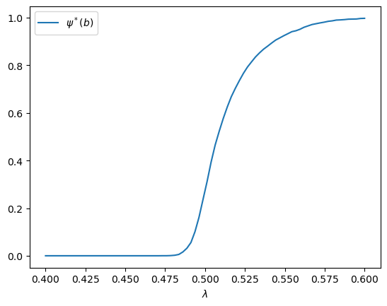
Now we address exercise 11.26.

We need to determine the fraction of time the sample spends at the point \(b\) in the state space over a long horizon, for different values of \(\lambda\).

grid_size = 80
lambdas = np.linspace(0.4, 0.6, grid_size)
mc_size = 5000

prob_at_b = np.empty_like(lambdas)

for i, lda in enumerate(lambdas):
    obs = generate_ts(lda, ts_length=mc_size)
    prob_at_b[i] = np.mean(obs == b)

fig, ax = plt.subplots()
ax.plot(lambdas, prob_at_b, label=r'$\psi^*({b})$')
ax.set_xlabel(r'$\lambda$')
ax.legend()

plt.show()