4. Working with Data#

In addition to what’s in Anaconda, this lecture needs the following library:

!pip install --upgrade wbgapi

4.1. Overview#

pandas is the standard library for working with tables of data in Python.

AI tools are trained on masses of pandas code, and most of what you do with AI and data in Python will involve substantial amounts of it.

As such, we at least need to understand the basics.

Just as NumPy provides the basic array data type plus core array operations, pandas

defines fundamental structures for working with data and
endows them with methods that facilitate operations such as
- reading in data
- adjusting indices
- working with dates and time series
- sorting, grouping, re-ordering and general data munging [1]
- dealing with missing values, etc., etc.

Note

pandas does not contain sophisticated statistical routines.

Rather, it is a tool for simple data analysis and a foundation for many other packages that work with pandas DataFrames, such as statsmodels and scikit-learn.

This lecture gives a fast-paced introduction to pandas.

We use the following imports.

import pandas as pd
import numpy as np
import matplotlib.pyplot as plt
from matplotlib.patches import FancyBboxPatch, Rectangle

4.2. Series#

Two important data types defined by pandas are Series and DataFrame.

You can think of a Series as a “column” of data, such as a collection of observations on a single variable.

A DataFrame is like a Series but it has multiple columns – analogous to a spreadsheet.

Let’s start with Series.

We begin by creating a series from a Python dictionary.

The keys are the ticker symbols of four listed companies, and the values are made-up daily returns on their shares, in percent.

returns = {'AMZN': 1.2, 'AAPL': -0.7, 'MSFT': 0.4, 'GOOG': -1.5}
s = pd.Series(returns, name='daily returns')
s

AMZN    1.2
AAPL   -0.7
MSFT    0.4
GOOG   -1.5
Name: daily returns, dtype: float64

The keys have become the index of the series.

Let’s compare this with a NumPy array containing the same numbers.

a = s.to_numpy()
a

array([ 1.2, -0.7,  0.4, -1.5])

The figure below shows the two side by side.

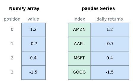
_images/3cf953c952ffccf30029ca56f623b5283c3e7844fb84e9b138620f90652545fa.png — Fig. 4.1 A NumPy array and a pandas Series#

We find a number in a NumPy array by its position.

print(a[0])

1.2

In a pandas series, we typically use its label.

print(s['AMZN'])

1.2

Series are built on top of NumPy arrays and support many similar operations.

For example, we can convert the returns from percentages to fractions.

s / 100

AMZN    0.012
AAPL   -0.007
MSFT    0.004
GOOG   -0.015
Name: daily returns, dtype: float64

We can also use NumPy functions

np.abs(s)

AMZN    1.2
AAPL    0.7
MSFT    0.4
GOOG    1.5
Name: daily returns, dtype: float64

But Series provide more than NumPy arrays.

For one thing, they have some additional (statistically oriented) methods

s.describe()

count    4.000000
mean    -0.150000
std      1.190238
min     -1.500000
25%     -0.900000
50%     -0.150000
75%      0.600000
max      1.200000
Name: daily returns, dtype: float64

And because of the index, Series are like Python dictionaries (with the restriction that the items in the dictionary all have the same type—in this case, floats).

In fact, you can use much of the same syntax as Python dictionaries

s['AMZN'] = 0
s

AMZN    0.0
AAPL   -0.7
MSFT    0.4
GOOG   -1.5
Name: daily returns, dtype: float64

'AAPL' in s

True

4.3. DataFrames#

While a Series is a single column of data, a DataFrame is several columns, one for each variable.

It is used to manage and analyze data that are naturally viewed as rows and columns.

Let’s look at an example that reads data from the CSV file gdp_population_by_country_2000.csv.

It holds data on seven countries in the year 2000, in the layout of the Penn World Tables.

The numbers are for illustration only, since they do not match any downloadable release of those tables.

The dataset contains the following indicators

Variable Name	Description
POP	Population (in thousands)
tcgdp	GDP (millions of international dollars)
cc	Consumption Share of GDP Per Capita (%)
cg	Government Consumption Share of GDP Per Capita (%)

We’ll read this in from a URL using the pandas function read_csv.

url = ('https://github.com/QuantEcon/data-lectures/raw/main/lectures/'
       'gdp_population_by_country_2000.csv')
df = pd.read_csv(url)
type(df)

pandas.DataFrame

Here’s the content of the file

df

	country	POP	tcgdp	cc	cg
0	Argentina	37335.653	2.950722e+05	75.716805	5.578804
1	Australia	19053.186	5.418047e+05	67.759026	6.720098
2	India	1006300.297	1.728144e+06	64.575551	14.072206
3	Israel	6114.570	1.292539e+05	64.436451	10.266688
4	Malawi	11801.505	5.026222e+03	74.707624	11.658954
5	South Africa	45064.098	2.272424e+05	72.718710	5.726546
6	United States	282171.957	9.898700e+06	72.347054	6.032454

The leftmost column, 0, 1, ..., 6, is the index of the DataFrame.

It is not in the file: pandas created it because the file does not supply one, and you will see this often when reading CSV files.

The country names make a more useful index, so let’s use them instead.

df = df.set_index('country')
df

	POP	tcgdp	cc	cg
country
Argentina	37335.653	2.950722e+05	75.716805	5.578804
Australia	19053.186	5.418047e+05	67.759026	6.720098
India	1006300.297	1.728144e+06	64.575551	14.072206
Israel	6114.570	1.292539e+05	64.436451	10.266688
Malawi	11801.505	5.026222e+03	74.707624	11.658954
South Africa	45064.098	2.272424e+05	72.718710	5.726546
United States	282171.957	9.898700e+06	72.347054	6.032454

The country names are now the index, and country is no longer one of the columns.

The figure below shows the parts of this DataFrame.

Show source

Hide code cell source

column_color = '#e8e3f4'
n = len(df)
index_width, width, gap = 3.1, 2.6, 0.35
x_index = 2.0
x_values = x_index + index_width + gap
x_end = x_values + 4 * width + 3 * gap
x_center = (x_values + x_end) / 2
header_y = n + 0.2


def draw_header(x, cell_width, name, color):
    "Draw a cell holding a name, above a column of cells."
    ax.add_patch(Rectangle((x, header_y), cell_width, 1, facecolor=color,
                           edgecolor=edge_color))
    ax.text(x + cell_width / 2, header_y + 0.5, name, ha='center', va='center')


def arrow(start, end):
    "Draw a thin arrow between two points."
    ax.annotate('', xy=end, xytext=start,
                arrowprops=dict(arrowstyle='-|>', color=muted_color, lw=1.2))


def label(x, y, text, **kwargs):
    "Write a label in the muted text color."
    ax.text(x, y, text, color=muted_color, ha='center', va='center', **kwargs)


fig, ax = plt.subplots(figsize=(8, 5))

# Positions are implicit, so they are not drawn as cells
for i in range(n):
    label(1.0, n - 0.5 - i, str(i))
label(1.0, header_y + 0.5, 'position', fontsize=8.5)

# The index
draw_cells(ax, x_index, index_width, df.index, index_color, '')
draw_header(x_index, index_width, df.index.name, index_color)
label(x_index + index_width / 2, -0.95, 'df.index', family='monospace')
arrow((x_index + index_width / 2, -0.65), (x_index + index_width / 2, -0.05))

# Each column is a Series with its own data type, and they share the index
for j, column in enumerate(df.columns):
    x = x_values + j * (width + gap)
    style = '{:,.0f}' if column in ('POP', 'tcgdp') else '{:.1f}'
    entries = [style.format(v) for v in df[column]]
    draw_cells(ax, x, width, entries, value_color, '')
    draw_header(x, width, column, column_color)
    ax.add_patch(FancyBboxPatch((x - 0.1, -0.12), width + 0.2, header_y + 1.24,
                                boxstyle='round,pad=0,rounding_size=0.18',
                                fill=False, linestyle='--',
                                edgecolor=muted_color))
    label(x + width / 2, -0.55, str(df[column].dtype),
          family='monospace', fontsize=8.5)
    ax.plot([x + width / 2, x_center], [header_y + 1.12, header_y + 2.0],
            ls=':', color=muted_color, lw=1)

label(x_center, header_y + 2.3, 'each column is a Series')

# The column labels
label(x_end + 2.15, header_y + 0.5, 'df.columns', family='monospace')
arrow((x_end + 0.9, header_y + 0.5), (x_end + 0.15, header_y + 0.5))

# The two axes
arrow((0.3, n), (0.3, 0.2))
label(-0.1, n / 2, 'axis=0', family='monospace', fontsize=8.5, rotation=90)
arrow((x_index + 1.0, header_y + 2.0), (x_index + 3.0, header_y + 2.0))
label(x_index + 0.25, header_y + 2.0, 'axis=1', family='monospace', fontsize=8.5)

ax.set_xlim(-0.4, x_end + 3.4)
ax.set_ylim(-1.3, header_y + 2.7)
ax.axis('off')
plt.show()

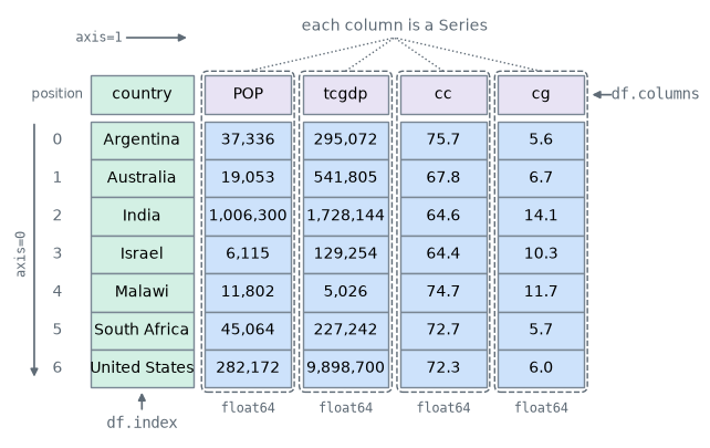
_images/e7657b8ec89ce96cbd3c078e08ed5f86e75c75c2643f9bfa4c47d81a0f108c24.png — Fig. 4.2 The parts of a DataFrame#

Each column is a Series with its own data type, and all the columns share the same index.

This figure, the earlier comparison of an array and a Series, and the merge figure below follow the diagrams in Lev Maximov’s Pandas Illustrated, which is a good visual guide to the library.

4.3.1. A first look at a dataset#

Seven rows fit on the screen, but most real datasets do not.

So the first step with a new dataset is usually to run a few standard checks.

The shape attribute gives the number of rows and columns.

df.shape

(7, 4)

The head method shows the first few rows.

df.head(3)

	POP	tcgdp	cc	cg
country
Argentina	37335.653	2.950722e+05	75.716805	5.578804
Australia	19053.186	5.418047e+05	67.759026	6.720098
India	1006300.297	1.728144e+06	64.575551	14.072206

The info method lists each column with its data type and its number of non-missing values.

df.info()

<class 'pandas.DataFrame'>
Index: 7 entries, Argentina to United States
Data columns (total 4 columns):
 #   Column  Non-Null Count  Dtype  
---  ------  --------------  -----  
 0   POP     7 non-null      float64
 1   tcgdp   7 non-null      float64
 2   cc      7 non-null      float64
 3   cg      7 non-null      float64
dtypes: float64(4)
memory usage: 340.0 bytes

The describe method gives summary statistics for each numeric column.

df.describe()

	POP	tcgdp	cc	cg
count	7.000000e+00	7.000000e+00	7.000000	7.000000
mean	2.011202e+05	1.832178e+06	70.323032	8.579393
std	3.681215e+05	3.603739e+06	4.697746	3.405579
min	6.114570e+03	5.026222e+03	64.436451	5.578804
25%	1.542735e+04	1.782481e+05	66.167289	5.879500
50%	3.733565e+04	2.950722e+05	72.347054	6.720098
75%	1.636180e+05	1.134975e+06	73.713167	10.962821
max	1.006300e+06	9.898700e+06	75.716805	14.072206

These checks catch many problems early, such as a column of numbers that was read in as text.

4.3.2. Select data by position and label#

In practice, one thing that we do all the time is to find, select and work with a subset of the data of our interests.

To select rows and columns by position, the iloc attribute should be used with the format .iloc[rows, columns].

df.iloc[2:5, 0:2]

	POP	tcgdp
country
India	1006300.297	1.728144e+06
Israel	6114.570	1.292539e+05
Malawi	11801.505	5.026222e+03

To select rows and columns by label, the loc attribute can be used in a similar way

df.loc[['India', 'Israel', 'Malawi'], ['POP', 'tcgdp']]

	POP	tcgdp
country
India	1006300.297	1.728144e+06
Israel	6114.570	1.292539e+05
Malawi	11801.505	5.026222e+03

We can also use it to pick out a single number

print(df.loc['India', 'POP'])

1006300.297

To select whole columns, we can pass a list containing their names

df[['POP', 'tcgdp']]

	POP	tcgdp
country
Argentina	37335.653	2.950722e+05
Australia	19053.186	5.418047e+05
India	1006300.297	1.728144e+06
Israel	6114.570	1.292539e+05
Malawi	11801.505	5.026222e+03
South Africa	45064.098	2.272424e+05
United States	282171.957	9.898700e+06

A single column is a Series, with the same index as the DataFrame

df['POP']

country
Argentina          37335.653
Australia          19053.186
India            1006300.297
Israel              6114.570
Malawi             11801.505
South Africa       45064.098
United States     282171.957
Name: POP, dtype: float64

For column names without spaces, df.POP does the same thing.

4.3.3. Select data by conditions#

Instead of indexing rows and columns using integers and names, we can also obtain a sub-dataframe of our interests that satisfies certain (potentially complicated) conditions.

This section demonstrates various ways to do that.

The most straightforward way is with the [] operator.

df[df.POP >= 20000]

	POP	tcgdp	cc	cg
country
Argentina	37335.653	2.950722e+05	75.716805	5.578804
India	1006300.297	1.728144e+06	64.575551	14.072206
South Africa	45064.098	2.272424e+05	72.718710	5.726546
United States	282171.957	9.898700e+06	72.347054	6.032454

To understand what is going on here, notice that df.POP >= 20000 returns a series of boolean values.

df.POP >= 20000

country
Argentina         True
Australia        False
India             True
Israel           False
Malawi           False
South Africa      True
United States     True
Name: POP, dtype: bool

In this case, df[___] takes a series of boolean values and only returns rows with the True values.

Take one more example,

df[df.index.isin(['Argentina', 'India', 'South Africa']) & (df.POP > 40000)]

	POP	tcgdp	cc	cg
country
India	1006300.297	1.728144e+06	64.575551	14.072206
South Africa	45064.098	2.272424e+05	72.718710	5.726546

In fact, there is another way of doing the same thing, with more natural syntax.

df.query("country in ['Argentina', 'India', 'South Africa'] and POP > 40000")

	POP	tcgdp	cc	cg
country
India	1006300.297	1.728144e+06	64.575551	14.072206
South Africa	45064.098	2.272424e+05	72.718710	5.726546

The string is a Python expression that pandas evaluates, when called with df.query.

The syntax inside the string is quite easy to read.

Here’s another example.

Consider this arithmetic operation between different columns.

df[(df.cc + df.cg >= 80) & (df.POP <= 20000)]

	POP	tcgdp	cc	cg
country
Malawi	11801.505	5026.221784	74.707624	11.658954

It becomes more readable if we use df.query.

df.query("cc + cg >= 80 and POP <= 20000")

	POP	tcgdp	cc	cg
country
Malawi	11801.505	5026.221784	74.707624	11.658954

We can also use df.query to select the country with the largest consumption share cc.

df.query("cc == cc.max()")

	POP	tcgdp	cc	cg
country
Argentina	37335.653	295072.21869	75.716805	5.578804

When selecting rows and columns together, we typically use .loc.

For example, in the following code the first argument is the condition and the second is the list of columns we want to return.

df.loc[(df.cc + df.cg >= 80) & (df.POP <= 20000), ['POP', 'tcgdp']]

	POP	tcgdp
country
Malawi	11801.505	5026.221784

We can save any selection to a file for further analysis.

df_subset = df[['POP', 'tcgdp']]
df_subset.to_csv('population_and_gdp.csv')

4.3.4. The apply method#

Another widely used pandas method is df.apply().

It applies a function to each row/column and returns a series.

This function can be some built-in functions like the max function, a lambda function, or a user-defined function.

Here is an example using the max function

df.apply(max)

POP      1.006300e+06
tcgdp    9.898700e+06
cc       7.571681e+01
cg       1.407221e+01
dtype: float64

This line of code applies the max function to each column.

A lambda function is often used with df.apply().

For example, this adds the consumption and government shares in each row

df.apply(lambda row: row.cc + row.cg, axis=1)

country
Argentina        81.295610
Australia        74.479124
India            78.647757
Israel           74.703139
Malawi           86.366579
South Africa     78.445257
United States    78.379508
dtype: float64

Note

For the .apply() method

axis = 0 – apply function to each column (variables)
axis = 1 – apply function to each row (observations)
axis = 0 is the default parameter

There is an easier way to add those two shares.

df.cc + df.cg

country
Argentina        81.295610
Australia        74.479124
India            78.647757
Israel           74.703139
Malawi           86.366579
South Africa     78.445257
United States    78.379508
dtype: float64

But apply is useful for more complex operations.

For example, suppose that a donor is deciding which countries can receive aid.

Its rule has two parts:

A country with at most 40 million people qualifies if its GDP per capita is below 10,000 dollars.
A country with more than 40 million people qualifies if its GDP per capita is below 5,000 dollars, because it has more domestic resources to draw on.

We can write this rule as a function that takes one row and returns True or False.

def eligible(row):
    # tcgdp is in millions and POP is in thousands
    gdp_percap = row.tcgdp * 1e3 / row.POP
    limit = 5000 if row.POP > 40_000 else 10_000
    return gdp_percap < limit

Applying this function to each row gives a series of boolean values.

df.apply(eligible, axis=1)

country
Argentina         True
Australia        False
India             True
Israel           False
Malawi            True
South Africa     False
United States    False
dtype: bool

We can use this series with .loc[] to select the eligible countries and the columns we want.

df.loc[df.apply(eligible, axis=1), ['POP', 'tcgdp']]

	POP	tcgdp
country
Argentina	37335.653	2.950722e+05
India	1006300.297	1.728144e+06
Malawi	11801.505	5.026222e+03

South Africa misses out because of its size, even though it is poorer than Argentina.

4.3.5. Make changes in DataFrames#

The ability to make changes in dataframes is important to generate a clean dataset for future analysis.

1. We can simply use .loc[] to specify the column that we want to modify, and assign values

For example, suppose we learn that the figure for India’s government share is unreliable.

We can mark it as missing, so that we don’t use it by accident.

df.loc['India', 'cg'] = np.nan
df

	POP	tcgdp	cc	cg
country
Argentina	37335.653	2.950722e+05	75.716805	5.578804
Australia	19053.186	5.418047e+05	67.759026	6.720098
India	1006300.297	1.728144e+06	64.575551	NaN
Israel	6114.570	1.292539e+05	64.436451	10.266688
Malawi	11801.505	5.026222e+03	74.707624	11.658954
South Africa	45064.098	2.272424e+05	72.718710	5.726546
United States	282171.957	9.898700e+06	72.347054	6.032454

2. We can use the .apply() method to modify rows/columns as a whole

For example, suppose we want to report GDP in billions rather than millions.

def update_row(row):
    # convert tcgdp from millions to billions
    row.tcgdp = row.tcgdp / 1000
    return row

df.apply(update_row, axis=1)

	POP	tcgdp	cc	cg
country
Argentina	37335.653	295.072219	75.716805	5.578804
Australia	19053.186	541.804652	67.759026	6.720098
India	1006300.297	1728.144375	64.575551	NaN
Israel	6114.570	129.253894	64.436451	10.266688
Malawi	11801.505	5.026222	74.707624	11.658954
South Africa	45064.098	227.242369	72.718710	5.726546
United States	282171.957	9898.700000	72.347054	6.032454

This returns a new DataFrame, so df itself is unchanged.

3. We can use the .map() method to modify all individual entries in the dataframe altogether.

# Round all decimal numbers to 2 decimal places
df.map(lambda x: round(x, 2))

	POP	tcgdp	cc	cg
country
Argentina	37335.65	295072.22	75.72	5.58
Australia	19053.19	541804.65	67.76	6.72
India	1006300.30	1728144.37	64.58	NaN
Israel	6114.57	129253.89	64.44	10.27
Malawi	11801.50	5026.22	74.71	11.66
South Africa	45064.10	227242.37	72.72	5.73
United States	282171.96	9898700.00	72.35	6.03

4.3.6. Missing values#

Real datasets usually have gaps, which pandas marks with NaN.

So far df has one, India’s government share, so let’s insert a few more.

for idx in list(zip([0, 3, 5, 6], [2, 3, 2, 3])):
    df.iloc[idx] = np.nan

df

	POP	tcgdp	cc	cg
country
Argentina	37335.653	2.950722e+05	NaN	5.578804
Australia	19053.186	5.418047e+05	67.759026	6.720098
India	1006300.297	1.728144e+06	64.575551	NaN
Israel	6114.570	1.292539e+05	64.436451	NaN
Malawi	11801.505	5.026222e+03	74.707624	11.658954
South Africa	45064.098	2.272424e+05	NaN	5.726546
United States	282171.957	9.898700e+06	72.347054	NaN

The zip() function here creates pairs of values from the two lists (i.e. [0,2], [3,3] …)

The first step is to find the gaps.

The isna method marks each missing value as True, and summing counts them in each column.

df.isna().sum()

POP      0
tcgdp    0
cc       2
cg       3
dtype: int64

One option is to drop every row that has a missing value.

df.dropna()

	POP	tcgdp	cc	cg
country
Australia	19053.186	541804.652100	67.759026	6.720098
Malawi	11801.505	5026.221784	74.707624	11.658954

Notice how much data this loses: only two of the seven countries remain.

Another option is to fill the gaps with a fixed value.

df.fillna(0)

	POP	tcgdp	cc	cg
country
Argentina	37335.653	2.950722e+05	0.000000	5.578804
Australia	19053.186	5.418047e+05	67.759026	6.720098
India	1006300.297	1.728144e+06	64.575551	0.000000
Israel	6114.570	1.292539e+05	64.436451	0.000000
Malawi	11801.505	5.026222e+03	74.707624	11.658954
South Africa	45064.098	2.272424e+05	0.000000	5.726546
United States	282171.957	9.898700e+06	72.347054	0.000000

This is clearly wrong here, since no country has a consumption share of zero.

A common alternative is single imputation, which fills each gap with the mean of its column.

df.fillna(df.mean())

	POP	tcgdp	cc	cg
country
Argentina	37335.653	2.950722e+05	68.765141	5.578804
Australia	19053.186	5.418047e+05	67.759026	6.720098
India	1006300.297	1.728144e+06	64.575551	7.421101
Israel	6114.570	1.292539e+05	64.436451	7.421101
Malawi	11801.505	5.026222e+03	74.707624	11.658954
South Africa	45064.098	2.272424e+05	68.765141	5.726546
United States	282171.957	9.898700e+06	72.347054	7.421101

None of these calls changes df, since each one returns a new DataFrame.

Missing value imputation is a big area in data science involving various machine learning techniques.

There are also more advanced tools in Python to impute missing values.

4.3.7. New columns, sorting and plotting#

For the rest of this section we only need population (POP) and total GDP (tcgdp), which have no gaps.

df = df[['POP', 'tcgdp']]
df

	POP	tcgdp
country
Argentina	37335.653	2.950722e+05
Australia	19053.186	5.418047e+05
India	1006300.297	1.728144e+06
Israel	6114.570	1.292539e+05
Malawi	11801.505	5.026222e+03
South Africa	45064.098	2.272424e+05
United States	282171.957	9.898700e+06

Let’s give the columns slightly better names

df.columns = 'population', 'total GDP'
df

	population	total GDP
country
Argentina	37335.653	2.950722e+05
Australia	19053.186	5.418047e+05
India	1006300.297	1.728144e+06
Israel	6114.570	1.292539e+05
Malawi	11801.505	5.026222e+03
South Africa	45064.098	2.272424e+05
United States	282171.957	9.898700e+06

The population variable is in thousands, let’s revert to single units

df['population'] = df['population'] * 1e3
df

	population	total GDP
country
Argentina	3.733565e+07	2.950722e+05
Australia	1.905319e+07	5.418047e+05
India	1.006300e+09	1.728144e+06
Israel	6.114570e+06	1.292539e+05
Malawi	1.180150e+07	5.026222e+03
South Africa	4.506410e+07	2.272424e+05
United States	2.821720e+08	9.898700e+06

Next, we’re going to add a column showing real GDP per capita, multiplying by 1,000,000 as we go because total GDP is in millions

df['GDP percap'] = df['total GDP'] * 1e6 / df['population']
df

	population	total GDP	GDP percap
country
Argentina	3.733565e+07	2.950722e+05	7903.229085
Australia	1.905319e+07	5.418047e+05	28436.433261
India	1.006300e+09	1.728144e+06	1717.324719
Israel	6.114570e+06	1.292539e+05	21138.672749
Malawi	1.180150e+07	5.026222e+03	425.896679
South Africa	4.506410e+07	2.272424e+05	5042.647686
United States	2.821720e+08	9.898700e+06	35080.381854

One of the nice things about pandas DataFrame and Series objects is that they have methods for plotting and visualization that work through Matplotlib.

For example, we can easily generate a bar plot of GDP per capita

ax = df['GDP percap'].plot(kind='bar')
ax.set_xlabel('country', fontsize=12)
ax.set_ylabel('GDP per capita', fontsize=12)
plt.show()

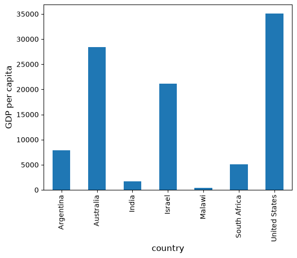
_images/212b8f4d585ce1aa2565172afa99792b997e49ef02fb3571e6d1b04079397ff9.png — Fig. 4.3 GDP per capita, in alphabetical order#

At the moment the data frame is ordered alphabetically on the countries—let’s change it to GDP per capita

df = df.sort_values(by='GDP percap', ascending=False)
df

	population	total GDP	GDP percap
country
United States	2.821720e+08	9.898700e+06	35080.381854
Australia	1.905319e+07	5.418047e+05	28436.433261
Israel	6.114570e+06	1.292539e+05	21138.672749
Argentina	3.733565e+07	2.950722e+05	7903.229085
South Africa	4.506410e+07	2.272424e+05	5042.647686
India	1.006300e+09	1.728144e+06	1717.324719
Malawi	1.180150e+07	5.026222e+03	425.896679

Plotting as before now yields

ax = df['GDP percap'].plot(kind='bar')
ax.set_xlabel('country', fontsize=12)
ax.set_ylabel('GDP per capita', fontsize=12)
plt.show()

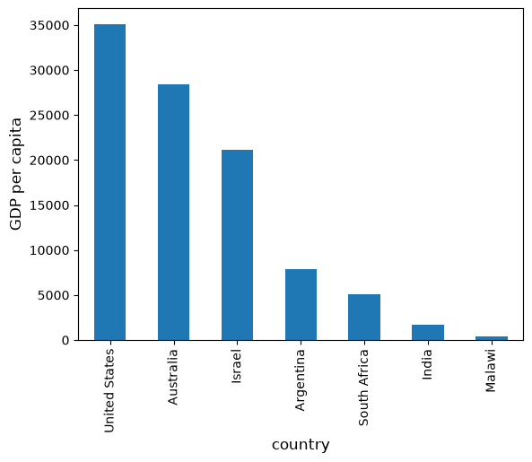
_images/fbefdb18e34f8c35418370610a5ebf3e3b45bc60175edcac603963d46bfb1002.png — Fig. 4.4 GDP per capita, sorted#

4.3.8. Merging and grouping#

Most real analyses combine data from more than one source.

Suppose we have a second table that assigns each country to a region.

regions = pd.DataFrame({
    'country': ['Argentina', 'Australia', 'India', 'Israel',
                'Malawi', 'South Africa', 'USA'],
    'region': ['Americas', 'Oceania', 'Asia', 'Asia',
               'Africa', 'Africa', 'Americas'],
})
regions

	country	region
0	Argentina	Americas
1	Australia	Oceania
2	India	Asia
3	Israel	Asia
4	Malawi	Africa
5	South Africa	Africa
6	USA	Americas

We can combine the two tables with merge, matching rows on the country name.

merged = df.merge(regions, on='country')
merged

	country	population	total GDP	GDP percap	region
0	Australia	1.905319e+07	5.418047e+05	28436.433261	Oceania
1	Israel	6.114570e+06	1.292539e+05	21138.672749	Asia
2	Argentina	3.733565e+07	2.950722e+05	7903.229085	Americas
3	South Africa	4.506410e+07	2.272424e+05	5042.647686	Africa
4	India	1.006300e+09	1.728144e+06	1717.324719	Asia
5	Malawi	1.180150e+07	5.026222e+03	425.896679	Africa

The result has country as an ordinary column again, with a new integer index.

Now look closely at the rows: the United States has disappeared.

The second table calls it USA, so the row has no match, and by default merge keeps only the rows that match.

No error or warning tells us this has happened.

One useful habit is to compare the number of rows before and after a merge.

print(len(df), len(merged))

7 6

Another is to use how='left', which keeps every row of the first table and shows the gap as NaN.

df.merge(regions, on='country', how='left')

	country	population	total GDP	GDP percap	region
0	United States	2.821720e+08	9.898700e+06	35080.381854	NaN
1	Australia	1.905319e+07	5.418047e+05	28436.433261	Oceania
2	Israel	6.114570e+06	1.292539e+05	21138.672749	Asia
3	Argentina	3.733565e+07	2.950722e+05	7903.229085	Americas
4	South Africa	4.506410e+07	2.272424e+05	5042.647686	Africa
5	India	1.006300e+09	1.728144e+06	1717.324719	Asia
6	Malawi	1.180150e+07	5.026222e+03	425.896679	Africa

The figure below shows both merges, with the unmatched rows highlighted.

Blue cells come from df and green cells come from regions.

Show source

Hide code cell source

unmatched_color = '#fbdccb'
source_colors = {'population': value_color, 'region': index_color}


def draw_cell(x, y, width, text, color):
    "Draw one table cell with its lower left corner at (x, y)."
    ax.add_patch(Rectangle((x, y), width, 1, facecolor=color,
                           edgecolor=edge_color))
    ax.text(x + width / 2, y + 0.5, text, ha='center', va='center', fontsize=9)


def as_text(frame):
    "Return a table of strings, with population in millions."
    table = frame.reset_index() if frame.index.name else frame.copy()
    if 'population' in table:
        table['population'] = (table['population'] / 1e6).map('{:,.1f}'.format)
    return table.fillna('NaN')


def merge_color(row, column):
    "Color each cell by its source table, and highlight unmatched rows."
    if row['country'] in ('United States', 'USA'):
        return unmatched_color
    return source_colors.get(column, 'white')


def draw_table(x, top, table, widths, title, cell_color):
    "Draw a table with its top left corner at (x, top)."
    ax.text(x, top + 0.45, title, family='monospace', fontsize=9, va='center')
    for j, column in enumerate(table.columns):
        left = x + sum(widths[:j])
        draw_cell(left, top - 1, widths[j], column, column_color)
        for i, entry in enumerate(table[column]):
            color = cell_color(table.iloc[i], column)
            draw_cell(left, top - 2 - i, widths[j], entry, color)


columns = ['country', 'population', 'region']
inner = as_text(df.merge(regions, on='country'))[columns]
left = as_text(df.merge(regions, on='country', how='left'))[columns]
wide = [3.1, 2.2, 2.2]

fig, ax = plt.subplots(figsize=(8, 6.8))

draw_table(1.0, 19, as_text(df[['population']]), [3.1, 2.2], 'df', merge_color)
draw_table(10.2, 19, regions, [3.1, 2.2], 'regions', merge_color)

draw_table(0, 8.6, inner, wide, "df.merge(regions, on='country')", merge_color)
label(3.75, 0.1, 'United States is dropped, with no warning', fontsize=9)

draw_table(8.7, 8.6, left, wide, "df.merge(regions, on='country', how='left')",
           merge_color)

arrow((3.6, 10.7), (3.6, 9.7))
arrow((12.45, 10.7), (12.45, 9.7))

ax.set_xlim(-0.1, 16.3)
ax.set_ylim(-0.4, 20)
ax.axis('off')
plt.show()

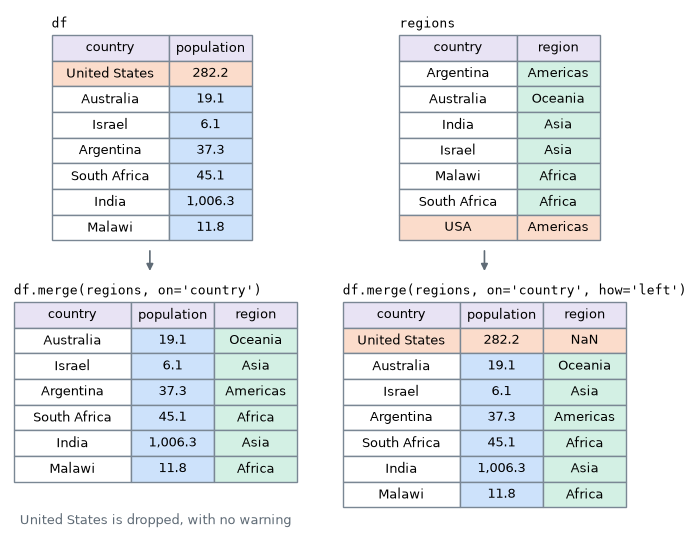
_images/b5f47f6480e53043316af62b7e7249fc74b46ce315814ab3a4288dbfb96e6ccf.png — Fig. 4.5 Two ways to merge, with population in millions#

Let’s fix the name and merge again.

regions['country'] = regions['country'].replace('USA', 'United States')
merged = df.merge(regions, on='country')
merged

	country	population	total GDP	GDP percap	region
0	United States	2.821720e+08	9.898700e+06	35080.381854	Americas
1	Australia	1.905319e+07	5.418047e+05	28436.433261	Oceania
2	Israel	6.114570e+06	1.292539e+05	21138.672749	Asia
3	Argentina	3.733565e+07	2.950722e+05	7903.229085	Americas
4	South Africa	4.506410e+07	2.272424e+05	5042.647686	Africa
5	India	1.006300e+09	1.728144e+06	1717.324719	Asia
6	Malawi	1.180150e+07	5.026222e+03	425.896679	Africa

Now we can use the new column with groupby, which splits the rows into groups and computes something for each one.

For example, here is the total population of each region, in millions.

merged.groupby('region')['population'].sum() / 1e6

region
Africa        56.865603
Americas     319.507610
Asia        1012.414867
Oceania       19.053186
Name: population, dtype: float64

The figure below shows the steps: the rows are split by region, each group is summed, and the results are combined into one table.

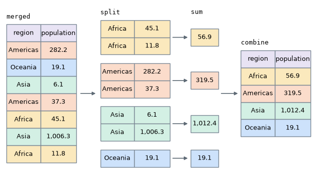
_images/bb695dce07d7e07723c2fe1382b59ee7ab15eb021282df57c5299f9c41655614.png — Fig. 4.6 Split, sum and combine, with population in millions#

4.3.9. Silent failures#

Code that runs without an error message can still give the wrong answer.

The merge that lost the United States is one example.

Here is another.

Suppose that Argentina’s population is missing, and that we fill the gap with the mean, just as we did for missing values above.

raw = pd.read_csv(url).set_index('country')
raw.loc['Argentina', 'POP'] = np.nan
filled = raw.fillna(raw.mean())

# tcgdp is in millions and POP is in thousands
gdp_percap = filled['tcgdp'] * 1e3 / filled['POP']

comparison = df[['GDP percap']].copy()
comparison['with imputed population'] = gdp_percap
comparison

	GDP percap	with imputed population
country
United States	35080.381854	35080.381854
Australia	28436.433261	28436.433261
Israel	21138.672749	21138.672749
Argentina	7903.229085	1291.810333
South Africa	5042.647686	5042.647686
India	1717.324719	1717.324719
Malawi	425.896679	425.896679

Argentina’s GDP per capita is now far too low, because India and the United States pull the mean population well above Argentina’s true population.

Nothing warned us: the code ran, the result looks like any other table, and no missing values remain to show that something was changed.

Filling in a missing value is a modeling choice, and every number computed from that value inherits its error.

4.4. Online data sources#

Someone has to collect every number that we analyze.

Most data used in policy work is produced by national statistical agencies, central banks and international organizations, using surveys, censuses and administrative records such as tax filings.

Before using a series, it is worth asking who produced it, how it was measured and whether it has been revised.

Many of these sources can be read directly from Python.

4.4.1. FRED#

FRED is a vast collection of time series data maintained by the St. Louis Fed.

For example, it holds the US unemployment rate, which the Bureau of Labor Statistics estimates from a monthly household survey.

Since read_csv accepts a URL, reading this series takes one line.

fred_url = 'https://fred.stlouisfed.org/graph/fredgraph.csv?id=UNRATE'
data = pd.read_csv(fred_url, index_col=0, parse_dates=True)
data.head()

	UNRATE
observation_date
1948-01-01	3.4
1948-02-01	3.8
1948-03-01	4.0
1948-04-01	3.9
1948-05-01	3.5

Here index_col=0 makes the first column the index, and parse_dates=True tells pandas that it holds dates.

Because the index holds dates, we can select a range of years with .loc.

ax = data.loc['2006':'2012'].plot(legend=False, lw=2)
ax.set_xlabel('year', fontsize=12)
ax.set_ylabel('unemployment rate (%)', fontsize=12)
plt.show()

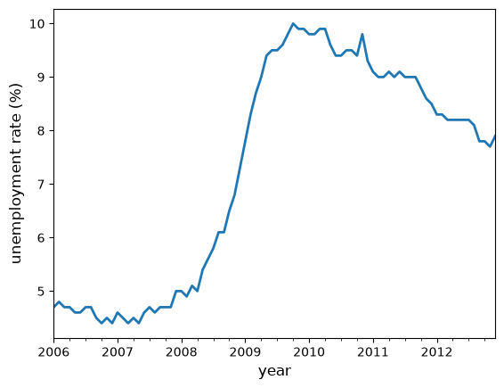
_images/dd4d2c8eb6f0bc76dcfff88de535eb7df3d1a3c62cc1c0786d73ecad1f20f0ce.png — Fig. 4.7 US unemployment rate#

pandas can also read many other formats, including Excel, JSON and Parquet files, and it can connect to databases.

4.4.2. The World Bank#

The World Bank collects and organizes data on a huge range of indicators.

The wbgapi library can fetch data from its databases, and this blog post gives an introduction.

For example, here’s some data on government debt as a ratio to GDP.

import wbgapi as wb
wb.series.info('GC.DOD.TOTL.GD.ZS')

id	value
GC.DOD.TOTL.GD.ZS	Central government debt, total (% of GDP)
	1 elements

The next code fetches the data and plots time series for the US and Australia.

govt_debt = wb.data.DataFrame('GC.DOD.TOTL.GD.ZS',
                              economy=['USA', 'AUS'],
                              time=range(2005, 2016))
govt_debt = govt_debt.T    # move years from columns to rows for plotting
ax = govt_debt.plot(lw=2)
ax.set_xlabel('year', fontsize=12)
ax.set_ylabel('government debt (% of GDP)', fontsize=12)
plt.show()

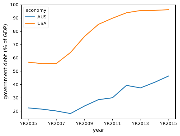
_images/0fa26e3278808c2fdf3d195279181b056163c1f82c8e6d676919a71ca973fc76.png — Fig. 4.8 Government debt as a ratio to GDP#

4.5. Exercises#

Exercise 4.1

You ask an AI tool to analyze the country data in gdp_population_by_country_2000.csv, and it returns the code below.

table = pd.read_csv(url).set_index('country')
table = table.query("cg > cg.mean()")
table = table.loc[:, ['POP', 'cg']].sort_values('cg', ascending=False)
table

Without running the code, say in one sentence what table it produces.

Then run it to check your answer.

Solution

The code lists the countries whose government share is above the average of the seven countries, showing their population and government share, with the largest share first.

table = pd.read_csv(url).set_index('country')
table = table.query("cg > cg.mean()")
table = table.loc[:, ['POP', 'cg']].sort_values('cg', ascending=False)
table

	POP	cg
country
India	1006300.297	14.072206
Malawi	11801.505	11.658954
Israel	6114.570	10.266688

Exercise 4.2

You ask an AI tool for the total GDP of each region, and it returns the code below.

gdp = pd.read_csv(url)
regions = pd.DataFrame({
    'country': ['Argentina', 'Australia', 'India', 'Israel', 'Israel',
                'Malawi', 'South Africa', 'United States'],
    'region': ['Americas', 'Oceania', 'Asia', 'Asia', 'Middle East',
               'Africa', 'Africa', 'Americas'],
})
merged = gdp.merge(regions, on='country')
merged.groupby('region')['tcgdp'].sum()

The code runs without an error.

Can you trust the answer?

Find the problem and fix it.

Solution

As in the lecture, we start by comparing the number of rows before and after the merge.

gdp = pd.read_csv(url)
regions = pd.DataFrame({
    'country': ['Argentina', 'Australia', 'India', 'Israel', 'Israel',
                'Malawi', 'South Africa', 'United States'],
    'region': ['Americas', 'Oceania', 'Asia', 'Asia', 'Middle East',
               'Africa', 'Africa', 'Americas'],
})
merged = gdp.merge(regions, on='country')
print(len(gdp), len(merged))

7 8

The merge has added a row, so some country must appear twice in regions.

regions[regions['country'].duplicated(keep=False)]

	country	region
3	Israel	Asia
4	Israel	Middle East

Israel is listed under two regions, so its GDP is counted twice and the regional totals add up to more than the total GDP of the seven countries.

print(gdp['tcgdp'].sum(), merged['tcgdp'].sum())

12825243.7310936 12954497.6253236

To fix this, we give each country one region.

Which region to use for Israel is a judgment call, and here we choose Asia.

We also pass validate='many_to_one', which makes merge raise an error if a country appears twice in regions.

regions = regions[regions['region'] != 'Middle East']
merged = gdp.merge(regions, on='country', validate='many_to_one')
merged.groupby('region')['tcgdp'].sum()

region
Africa      2.322686e+05
Americas    1.019377e+07
Asia        1.857398e+06
Oceania     5.418047e+05
Name: tcgdp, dtype: float64

Exercise 4.3

Using the corrected merged table from Exercise 4.2, compute GDP per capita for each region in two ways:

the average of GDP per capita across the countries in the region
the total GDP of the region divided by its total population

You can write this yourself or ask an AI tool to do it.

Why are the two answers so different for Asia?

Which one would you report, and when?

Solution

Here is one way to compute both.

merged['gdp_percap'] = merged['tcgdp'] * 1e3 / merged['POP']
average = merged.groupby('region')['gdp_percap'].mean()

totals = merged.groupby('region')[['tcgdp', 'POP']].sum()
whole_region = totals['tcgdp'] * 1e3 / totals['POP']

pd.DataFrame({'average of countries': average,
              'region as a whole': whole_region})

	average of countries	region as a whole
region
Africa	2734.272182	4084.518215
Americas	21491.805469	31904.630436
Asia	11427.998734	1834.621685
Oceania	28436.433261	28436.433261

The average of countries gives India and Israel equal weight, even though India has more than 160 times as many people.

The second number is close to India’s own figure, because India makes up nearly all of the region’s population.

Neither answer is wrong, because they answer different questions, as in Reading Python and Directing AI.

The first describes a typical country, while the second describes the income of a typical person.