7. Bivariate Distributions, Correlation and Simple Regression#
7.1. Outline#
The lectures Probability Distributions and Observed Distributions and Matching Them to Data study a single variable at a time (e.g., a distribution of house prices).
Often we are interested in how two variables relate to each other.
For example, do larger houses tend to sell for more?
In this lecture we study joint distributions and correlation, and then fit a line through data using regression.
We end with a warning about what such a line can and cannot tell us.
We use the following imports:
import os

import matplotlib.pyplot as plt
import pandas as pd
import numpy as np
import scipy.stats
from scipy.optimize import minimize
import seaborn as sns

np.set_printoptions(legacy='1.25')   # print scalars as plain numbers
To motivate what follows, let’s look at the sale prices and floor areas of the Ames houses that we studied in Observed Distributions and Matching Them to Data.
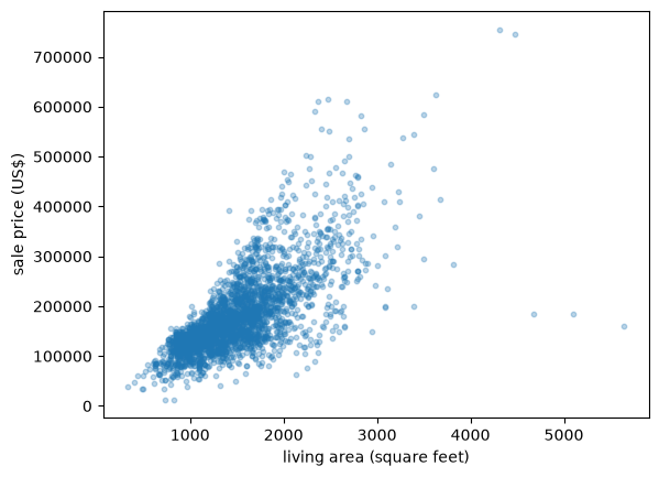
Fig. 7.1 House price against floor area#
Each point is one house, and larger houses clearly tend to sell for more.
This is the kind of pattern that a joint distribution can describe.
7.2. Joint and marginal distributions#
We start with the discrete case and then turn to densities.
7.2.1. Discrete case#
Let \(X\) and \(Y\) be two discrete random variables, taking values in finite sets \(S_X\) and \(S_Y\).
Their joint distribution is described by the function
As with a single variable, the values of \(p\) are nonnegative and sum to one, now over both variables.
Let’s build an example from the house price data.
Let \(X = 1\) if a house’s floor area is above the sample mean and \(X=0\) otherwise, and define \(Y\) the same way for price.
X = (area > area.mean()).astype(int)
Y = (price > price.mean()).astype(int)
joint = pd.crosstab(X, Y, normalize=True)
joint.index.name = 'x (area above mean)'
joint.columns.name = 'y (price above mean)'
joint
| y (price above mean) | 0 | 1 |
|---|---|---|
| x (area above mean) | ||
| 0 | 0.479522 | 0.073038 |
| 1 | 0.137201 | 0.310239 |
Each cell is the fraction of houses with that combination of \(X\) and \(Y\).
Around 48% of houses have both below-mean floor area and below-mean price.
Given a joint distribution, we can recover the distribution of \(X\) on its own by summing out \(Y\):
and symmetrically for \(p_Y\).
We call \(p_X\) and \(p_Y\) the marginal distributions of \(X\) and \(Y\).
In our table, the marginals are the row and column sums:
p_X, p_Y = joint.sum(axis=1), joint.sum(axis=0)
p_X, p_Y
(x (area above mean)
 0    0.55256
 1    0.44744
 dtype: float64,
 y (price above mean)
 0    0.616724
 1    0.383276
 dtype: float64)
Notice that the marginals alone do not tell us the whole story.
Knowing the fraction of houses with above-mean area and the fraction with above-mean price, separately, says nothing about whether the same houses tend to have both.
For that we need the joint distribution.
7.2.2. Continuous case#
Some variables are continuous rather than discrete.
The continuous analog is the joint density \(p(x,y)\), a nonnegative function on \(\mathbb R^2\) with
We say that \((X,Y)\) has joint density \(p\) if, for every region \(A \subset \mathbb R^2\),
Marginal densities come from integrating out the other variable:
7.3. The bivariate normal distribution#
Just as the normal distribution is the workhorse univariate distribution, the bivariate normal distribution is the workhorse joint distribution.
It has five parameters: the two means \(\mu_X, \mu_Y\), the two standard deviations \(\sigma_X, \sigma_Y\), and the correlation \(\rho \in (-1,1)\), which we define below.
Its density is
SciPy provides this distribution as scipy.stats.multivariate_normal, which takes a mean and a covariance matrix.
def bivariate_normal(μ_x, μ_y, σ_x, σ_y, ρ):
    cov = [[σ_x**2, ρ * σ_x * σ_y],
           [ρ * σ_x * σ_y, σ_y**2]]
    return scipy.stats.multivariate_normal([μ_x, μ_y], cov)
Here is the density as a surface over the \((x,y)\) plane.
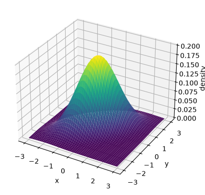
Fig. 7.2 The bivariate normal density surface#
This is the same kind of bell-shaped hill as the univariate normal density, built over a plane instead of a line.
It is usually more convenient to look straight down at the hill and draw its contour lines, the way a topographic map does.
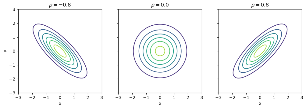
Fig. 7.3 Bivariate normal contours by correlation#
When \(\rho = 0\) the contours are circles, and otherwise they are tilted ellipses.
It can be shown that the marginal of \(X\) is \(N(\mu_X, \sigma_X^2)\) and the marginal of \(Y\) is \(N(\mu_Y, \sigma_Y^2)\).
Neither marginal depends on \(\rho\): the correlation describes how \(X\) and \(Y\) move together, and that information is lost when we look at either variable alone.
7.4. Independence and correlation#
\(X\) and \(Y\) are independent if the joint distribution is the product of the marginals:
Independence means that learning the value of \(X\) tells us nothing about \(Y\).
Let’s compare our house table with the table we would get if \(X\) and \(Y\) were independent.
independent_table = pd.DataFrame(np.outer(p_X, p_Y),
                                 index=joint.index, columns=joint.columns)

fig, axes = plt.subplots(1, 2, figsize=(9, 4))
for ax, table, title in zip(axes, (joint, independent_table),
                            ('actual joint', 'if independent')):
    sns.heatmap(table, annot=True, fmt='.2f', cmap='viridis', cbar=False,
                vmin=0, vmax=0.5, ax=ax)
    ax.set_title(title)
    ax.invert_yaxis()
plt.show()
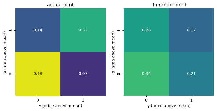
Fig. 7.4 Actual joint versus independent joint#
Around 48% of houses land in the (below, below) cell, well above the 34% that independence would predict.
So \(X\) and \(Y\) are far from independent, as we would expect, since larger houses tend to be more expensive.
Independence is an all-or-nothing property.
To measure the strength and direction of dependence, we use the covariance
The covariance is positive when \(X\) and \(Y\) tend to be above their means together, and negative when one tends to be above its mean while the other is below.
If \(X\) and \(Y\) are independent, then \(\mathrm{Cov}(X,Y) = 0\).
Note
The converse is false: zero covariance does not imply independence.
It only rules out linear dependence, as Exercise 7.3 shows.
The covariance is measured in the units of \(X\) times the units of \(Y\), which makes it hard to interpret.
We therefore usually standardize it into the correlation coefficient
Correlation is unit-free and always lies in \([-1, 1]\), with the extreme values attained only when \(Y\) is an exact linear function of \(X\).
For the bivariate normal, \(\rho\) is exactly this correlation, and \(\rho = 0\) implies independence, which is not true of distributions in general.
To estimate correlation from data \(\{(x_i, y_i)\}\), we replace population quantities with sample ones, which gives the sample correlation
where \(s_x\) and \(s_y\) are the sample standard deviations.
The function np.corrcoef returns a matrix of correlations, and we use [0, 1] to pull out the one between its two arguments.
np.corrcoef(area, price)[0, 1]
0.7067799209766282
7.5. Building joint distributions#
Why do two variables end up correlated?
A very common mechanism is that \(Y\) is built partly from \(X\):
where \(W\) is noise, independent of \(X\), with mean zero and standard deviation \(\sigma_W\).
Since \(W\) is independent of \(X\), we have \(\mathrm{Cov}(X,Y) = a \sigma_X^2\) and \(\mathbb V[Y] = a^2 \sigma_X^2 + \sigma_W^2\), so that
The correlation is driven entirely by the relative size of the signal \(a X\) and the noise \(W\).
Let’s see this in a picture, fixing \(a=1\) and \(\sigma_X = 1\) and increasing \(\sigma_W\).
rng = np.random.default_rng(1234)
N = 500
a = 1.0

fig, axes = plt.subplots(1, 3, figsize=(12, 4), sharex=True, sharey=True)
for ax, σ_w in zip(axes, (0.2, 1.0, 3.0)):
    x = rng.standard_normal(N)
    w = rng.normal(scale=σ_w, size=N)
    y = a * x + w
    ρ = a / np.sqrt(a**2 + σ_w**2)
    ax.scatter(x, y, alpha=0.5, s=10)
    ax.set_title(rf'$\sigma_W={σ_w}$, $\rho={ρ:.2f}$')
    ax.set_xlabel('x')
axes[0].set_ylabel('y')
plt.show()
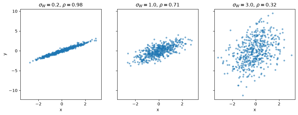
Fig. 7.5 Correlation falls as noise grows#
As the noise grows, the cloud of points fattens and the correlation falls, even though the underlying mechanism never changes.
If \(X\) and \(W\) are both normal, then the pair \((X,Y)\) built this way is bivariate normal.
7.6. When is a pair jointly normal?#
It is tempting to think that, if \(X\) and \(Y\) are each individually normal, then the pair \((X,Y)\) must be bivariate normal.
This is false.
Let \(X\) be standard normal, and construct \(Y\) by
Since the standard normal density is symmetric about zero, flipping the sign of \(X\) whenever \(|X| \geq 1\) does not change its distribution, so \(Y\) is also standard normal.
N = 2000
x = rng.standard_normal(N)
y = np.where(np.abs(x) < 1, x, -x)

g = sns.jointplot(x=x, y=y, height=5, alpha=0.4, s=8)
g.set_axis_labels('x', 'y')
plt.show()
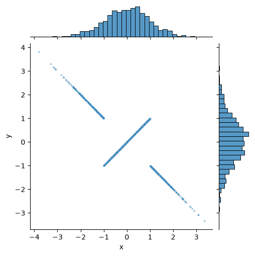
Fig. 7.6 Normal marginals, but not jointly normal#
The histograms on the margins have the familiar bell shape, yet the joint distribution looks nothing like an elliptical cloud.
It is concentrated on two crossing lines.
For a genuinely bivariate normal pair, every linear combination \(aX+bY\) is normal, but here \(X+Y = 0\) whenever \(|X| \geq 1\), which happens about a third of the time.
The lesson is that checking each variable individually is not enough: we need to look at the joint distribution directly.
7.7. Simple regression#
We now turn to fitting a line through data.
Let’s take a small data set in which \(y_i\) is the daily sales of an ice-cream cart in dollars and \(x_i\) is the day’s temperature in Celsius.
sales = pd.DataFrame({
    'temperature': [32, 21, 24, 35, 10, 11, 22, 21, 27, 2],
    'sales': [2000, 1000, 1500, 2500, 500, 900, 1100, 1500, 1800, 250]
})
x, y = sales['temperature'], sales['sales']
We would like to choose a line
that fits these data well.
7.7.1. Fitting by hand#
Let’s try two guesses, with the distance from each point to the line drawn in red.
def plot_fit(ax, α, β, label):
    "Plot the sales data, the line and the residuals."
    ax.scatter(x, y)
    x_vals = np.array([x.min(), x.max()])
    ax.plot(x_vals, α + β * x_vals, 'g', lw=2, label=label)
    ax.vlines(x, α + β * x, y, color='r', lw=1)
    ax.set_xlabel('temperature (Celsius)')
    ax.set_ylabel('sales (US$)')
    ax.legend()

fig, axes = plt.subplots(1, 2, figsize=(10, 4), sharey=True)
plot_fit(axes[0], 5, 10, r'$\alpha=5, \beta=10$')
plot_fit(axes[1], 5, 65, r'$\alpha=5, \beta=65$')
plt.show()
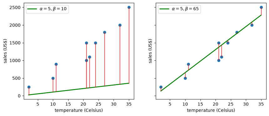
Fig. 7.7 Two lines fitted by hand#
The first line is poor and the second looks reasonable.
But which line is best depends on what we mean by “best”, so we need a criterion.
7.7.2. Choosing a criterion#
The red segments are the residuals
and a good line should make them small.
The most common criterion, called ordinary least squares (OLS), minimizes the sum of squared residuals
7.7.3. Optimizing#
Setting the partial derivatives of \(C\) to zero gives two equations, which we solve in Exercise 7.1.
The solution is
So the slope is the sample correlation \(r\), rescaled by the units of the two variables.
r = np.corrcoef(x, y)[0, 1]
β_hat = r * y.std() / x.std()
α_hat = y.mean() - β_hat * x.mean()
α_hat, β_hat
(-14.721485411140975, 64.3766578249337)
The function np.polyfit gives the same answer, with the slope first.
np.polyfit(x, y, 1)
array([ 64.37665782, -14.72148541])
Let’s confirm that these values really do minimize the criterion, by varying one parameter at a time.
def ssr(α, β):
    return ((y - α - β * x)**2).sum()

β_vals = np.linspace(20, 100, 200)
α_vals = np.linspace(-500, 500, 200)

fig, axes = plt.subplots(1, 2, figsize=(10, 4))
axes[0].plot(β_vals, [ssr(α_hat, β) for β in β_vals], lw=2)
axes[0].axvline(β_hat, color='r')
axes[0].set_xlabel(r'$\beta$')
axes[0].set_ylabel('sum of squared residuals')
axes[1].plot(α_vals, [ssr(α, β_hat) for α in α_vals], lw=2)
axes[1].axvline(α_hat, color='r')
axes[1].set_xlabel(r'$\alpha$')
plt.show()
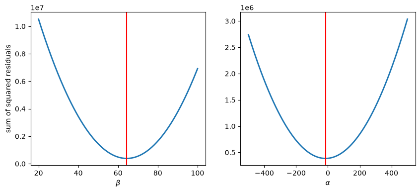
Fig. 7.8 The sum of squared residuals around the optimum#
7.7.4. Regression and the conditional mean#
For a bivariate normal pair, the best guess of \(Y\) given that \(X = x\) is a straight line in \(x\):
This has the same form as the OLS line, with \(\hat \alpha + \hat \beta x = \bar y + r (s_y / s_x)(x - \bar x)\).
So OLS estimates the conditional mean when the data are bivariate normal, and it remains a useful summary of a linear relationship when they are not.
Let’s fit a line to the house data, in logs, which makes both variables closer to normal.
log_area, log_price = np.log(area), np.log(price)
slope, intercept = np.polyfit(log_area, log_price, 1)
x_vals = np.array([log_area.min(), log_area.max()])

fig, ax = plt.subplots()
ax.scatter(log_area, log_price, alpha=0.2, s=8)
ax.plot(x_vals, intercept + slope * x_vals, 'k--', lw=2, label='OLS line')
ax.set_xlabel('log(living area)')
ax.set_ylabel('log(sale price)')
ax.legend()
plt.show()
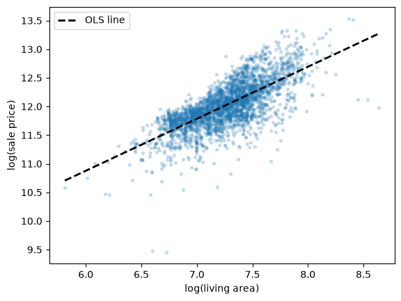
Fig. 7.9 Log price against log area, with the OLS line#
7.8. Other criteria#
Least squares is not the only reasonable criterion.
Squaring means that a large residual counts very heavily, so a single unusual observation can pull the whole line towards it.
An alternative is least absolute deviations (LAD), which minimizes
This criterion has no simple formula, so we minimize it numerically with SciPy.
To compare the two, suppose that we add one unusual day to the ice-cream data: a hot day when the cart broke down and sales were only 100 dollars.
x_new = np.append(x, 30)
y_new = np.append(y, 100)

def lad(p):
    α, β = p
    return np.abs(y_new - α - β * x_new).sum()

result = minimize(lad, x0=[0, 50], method='Nelder-Mead',
                  options={'xatol': 1e-3, 'fatol': 1e-3, 'maxiter': 4000})
α_lad, β_lad = result.x
β_ols, α_ols = np.polyfit(x_new, y_new, 1)

x_vals = np.array([x_new.min(), x_new.max()])

fig, ax = plt.subplots()
ax.scatter(x_new, y_new)
ax.scatter(30, 100, color='r', label='outlier')
ax.plot(x_vals, α_ols + β_ols * x_vals, lw=2, label='OLS')
ax.plot(x_vals, α_lad + β_lad * x_vals, lw=2, label='LAD')
ax.set_xlabel('temperature (Celsius)')
ax.set_ylabel('sales (US$)')
ax.legend()
plt.show()
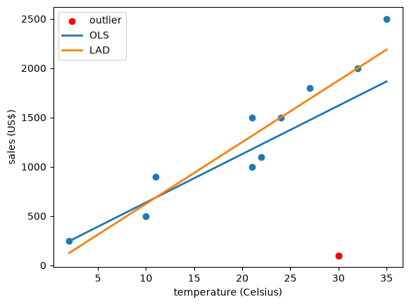
Fig. 7.10 OLS and LAD lines with an outlier#
β_ols, β_lad
(49.06388642413486, 62.50000787808858)
One bad day pulls the OLS slope down from about 64 to about 49, while the LAD slope stays at about 62.5, as it was without the outlier.
This is the same contrast as between the mean and the median in Observed Distributions and Matching Them to Data, and indeed LAD estimates the conditional median rather than the conditional mean.
7.9. An extended example#
Let’s use regression on a question of policy interest: how does life expectancy vary with income across countries?
The data come from Our World in Data, and we use 2018, the most recent year available.
url = ('https://github.com/QuantEcon/data-lectures/raw/main/'
       'lectures/life-expectancy-vs-gdp-per-capita.csv')
columns = ['Code', 'Year', 'Life expectancy at birth (historical)',
           'GDP per capita']
gdp_life = pd.read_csv(url, usecols=columns)[columns].dropna()
gdp_life.columns = ['code', 'year', 'life_expectancy', 'gdppc']

# keep 2018, and drop the world aggregate, which is not a country
gdp_life = gdp_life[(gdp_life['year'] == 2018)
                    & ~gdp_life['code'].str.startswith('OWID')]
gdp_life['log_gdppc'] = np.log10(gdp_life['gdppc'])
len(gdp_life)
165
Here are the data, with GDP per capita on both its original scale and a log scale.
slope, intercept = np.polyfit(gdp_life['log_gdppc'],
                              gdp_life['life_expectancy'], 1)
x_vals = np.array([gdp_life['log_gdppc'].min(), gdp_life['log_gdppc'].max()])

fig, axes = plt.subplots(1, 2, figsize=(10, 4), sharey=True)
axes[0].scatter(gdp_life['gdppc'], gdp_life['life_expectancy'], s=12, alpha=0.6)
axes[0].set_xticks(np.arange(0, 200_000, 50_000))
axes[0].set_xlabel('GDP per capita')
axes[0].set_ylabel('life expectancy (years)')
axes[1].scatter(gdp_life['log_gdppc'], gdp_life['life_expectancy'],
                s=12, alpha=0.6)
axes[1].plot(x_vals, intercept + slope * x_vals, 'k--', lw=2)
axes[1].set_xlabel('log10 of GDP per capita')
plt.show()
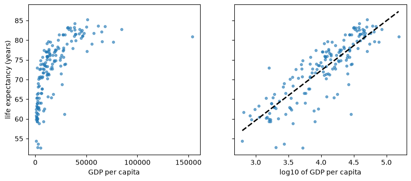
Fig. 7.11 Life expectancy against GDP per capita, 2018#
On the original scale the relationship is strongly curved, a pattern known as the Preston curve.
Taking logs makes it close to linear, so a straight line is a much better summary.
The correlation rises accordingly.
np.corrcoef(gdp_life['gdppc'], gdp_life['life_expectancy'])[0, 1], \
np.corrcoef(gdp_life['log_gdppc'], gdp_life['life_expectancy'])[0, 1]
(0.6658824887200563, 0.8437997115856368)
slope
12.65065681435222
Since we used base 10 logs, the slope says that a country with ten times the GDP per capita has, on average, about 13 more years of life expectancy.
Notice how carefully that sentence is worded, since it describes a pattern across countries and not the effect of raising a country’s income.
7.10. Correlation and causality#
Suppose a survey finds that women who own horses live longer than women who don’t.
It would be odd to prescribe horses for longevity.
Owning a horse is expensive, so horse owners are likely to be wealthier and to have better health insurance, and those may be what matters.
A third factor that affects both variables like this is called a confounder, and it can produce a correlation without any causal link between the two.
Here is a real example, using data on the 50 US states and the District of Columbia (DC).
For each one we have Donald Trump’s percentage share of the 2024 presidential vote, from the Federal Election Commission, and life expectancy at birth in 2021, from the US National Center for Health Statistics.
path = '_static/lecture_specific/bivariate_dist/state_votes_life_expectancy.csv'
url = ('https://raw.githubusercontent.com/jstac/py_for_ds_public/main/lectures/'
       + path)

# use the copy stored with this book if there is one, and otherwise download it
states = pd.read_csv(path if os.path.exists(path) else url)
states.head()
| state | code | trump_share | life_expectancy | |
|---|---|---|---|---|
| 0 | Alabama | AL | 64.57 | 72.0 |
| 1 | Alaska | AK | 54.54 | 74.5 |
| 2 | Arizona | AZ | 52.22 | 75.0 |
| 3 | Arkansas | AR | 64.20 | 72.5 |
| 4 | California | CA | 38.33 | 78.3 |
Let’s plot the data.
fig, ax = plt.subplots()
ax.scatter(states['trump_share'], states['life_expectancy'], alpha=0.7)
for _, row in states[states['code'].isin(['DC', 'HI', 'MS'])].iterrows():
    ax.annotate(row['code'], (row['trump_share'], row['life_expectancy']),
                xytext=(5, 5), textcoords='offset points')
ax.margins(y=0.1)
ax.set_xlabel('Trump share of the 2024 vote (%)')
ax.set_ylabel('life expectancy in 2021 (years)')
plt.show()
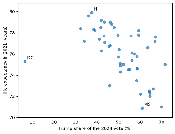
Fig. 7.12 Life expectancy against Trump vote share, by state#
DC sits far to the left of everything else, and it is a single city rather than a state, so let’s see what happens without it.
no_dc = states[states['code'] != 'DC']

r_all = np.corrcoef(states['trump_share'], states['life_expectancy'])[0, 1]
r_no_dc = np.corrcoef(no_dc['trump_share'], no_dc['life_expectancy'])[0, 1]
slope, intercept = np.polyfit(no_dc['trump_share'], no_dc['life_expectancy'], 1)

r_all, r_no_dc, slope
(-0.5300334565412842, -0.6567215590038358, -0.15599953282456586)
x_vals = np.array([no_dc['trump_share'].min(), no_dc['trump_share'].max()])

fig, ax = plt.subplots()
ax.scatter(no_dc['trump_share'], no_dc['life_expectancy'], alpha=0.7)
ax.plot(x_vals, intercept + slope * x_vals, 'k--', lw=2)
ax.set_xlabel('Trump share of the 2024 vote (%)')
ax.set_ylabel('life expectancy in 2021 (years)')
plt.show()
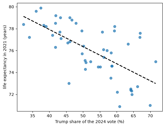
Fig. 7.13 The same data without DC, with the OLS line#
The correlation is about \(-0.53\) with DC and \(-0.66\) without it, so this one choice about the data matters, and any report should state it.
Without DC, states with a vote share 10 percentage points higher have life expectancy about 1.6 years lower, on average.
What can we conclude from this?
Not that voting one way or the other affects how long people live, since these data cannot tell us that.
Many factors differ across states and are related to both variables, including income, education, age, smoking, health insurance and region.
The year 2021 also falls in the pandemic, whose effects differed across states.
Moreover, each point is a whole state, so the figure says nothing directly about individuals, and in particular it does not show that any individual’s vote is related to their lifespan.
Drawing conclusions about individuals from group data like this is called the ecological fallacy.
Learning about causes takes more than a strong correlation: it takes a research design, such as a randomized trial, that rules out explanations like these.
7.11. Exercises#
Exercise 7.1
Derive the OLS formulas given above, by setting the partial derivatives of \(C(\alpha, \beta)\) to zero.
Solution
Setting the derivative with respect to \(\alpha\) to zero and dividing by \(-2\) gives
Dividing by \(n\) and rearranging gives \(\alpha = \bar y - \beta \bar x\).
Setting the derivative with respect to \(\beta\) to zero and dividing by \(-2\) gives
Substituting for \(\alpha\) gives
Since \(\sum_i (y_i - \bar y) = 0\) and \(\sum_i (x_i - \bar x) = 0\), we can subtract \(\bar x\) from \(x_i\) on both sides without changing either sum, which gives
Dividing the numerator and denominator by \(n\) shows that this equals \(r s_x s_y / s_x^2 = r s_y / s_x\).
Exercise 7.2
You ask an AI tool how much life expectancy rises with GDP per capita, using the gdp_life data above, and it returns the code below.
slope, intercept = np.polyfit(gdp_life['life_expectancy'],
                              gdp_life['log_gdppc'], 1)
print(slope)
It then reports that a tenfold rise in GDP per capita goes with about 0.056 more years of life expectancy.
The code runs without an error, but what is wrong?
Is the slope of one regression simply the inverse of the slope of the other?
Solution
The arguments are the wrong way around: np.polyfit takes \(x\) first, so this code regresses log GDP per capita on life expectancy.
wrong, _ = np.polyfit(gdp_life['life_expectancy'], gdp_life['log_gdppc'], 1)
right, _ = np.polyfit(gdp_life['log_gdppc'], gdp_life['life_expectancy'], 1)
wrong, right, 1 / right
(0.05628150093078481, 12.65065681435222, 0.07904727909980896)
The slope that the AI tool found is in units of log GDP per capita per year of life expectancy, so its statement is wrong.
The two slopes are also not inverses of each other, because the two regressions minimize different things: vertical distances in one case and horizontal distances in the other.
In fact their product is \(r^2\), so they would be inverses only if the points lay exactly on a line.
Exercise 7.3
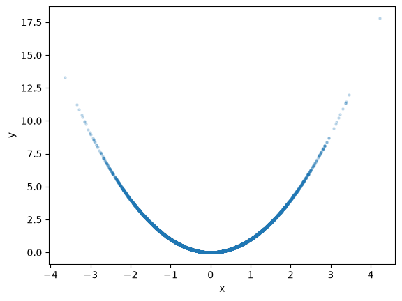
Let \(X\) be standard normal and let \(Y = X^2\).
Simulate a large sample, plot it and compute the sample correlation.
Are \(X\) and \(Y\) independent?
What does this tell us about reading a correlation close to zero?
Solution
x_sim = rng.standard_normal(10_000)
y_sim = x_sim**2

fig, ax = plt.subplots()
ax.scatter(x_sim, y_sim, alpha=0.2, s=5)
ax.set_xlabel('x')
ax.set_ylabel('y')
plt.show()

np.corrcoef(x_sim, y_sim)[0, 1]
0.00981053811951092
The correlation is close to zero, and indeed the population covariance is \(\mathbb E[X^3] = 0\).
Yet \(X\) and \(Y\) are far from independent, since \(X\) determines \(Y\) exactly.
Correlation only measures linear dependence, so we should always look at the data as well as the number.