3. The Toolkit: What Is Possible#
In this lecture we look at the hardware that runs our code, and then take a visual tour of what Python’s main libraries can do.
You do not need to memorize any of the code.
The aim is to know what is possible, so that you can ask an AI for it and judge what comes back.
Most of the code behind the figures is hidden, and you can click to show it.
In addition to what’s in Anaconda, this lecture needs JAX, which we discuss below, and a library containing the trade data that we use.
!pip install jax
!pip install quantecon_book_networks
We use these imports.
import json
import os
import urllib.request

import jax
import jax.numpy as jnp
import matplotlib.dates as mdates
import matplotlib.pyplot as plt
import networkx as nx
import numpy as np
import pandas as pd
import plotly.express as px
import seaborn as sns
import statsmodels.api as sm
from matplotlib.collections import PolyCollection
from matplotlib.colors import LinearSegmentedColormap
from matplotlib.patches import Rectangle
from scipy.integrate import quad
from scipy.stats import norm
from sklearn.cluster import KMeans
import quantecon_book_networks.data as qbn_data
import quantecon_book_networks.input_output as qbn_io

# Colors used in the figures below
blue, orange, aqua, yellow = '#2a78d6', '#eb6834', '#1baf7a', '#eda100'
blues = LinearSegmentedColormap.from_list(
    'blues', ['#cde2fb', '#6da7ec', '#2a78d6', '#184f95', '#0d366b'])
3.1. Hardware#
Data science increasingly depends on specialized hardware, so we start with the basic parts of a computer.
3.1.1. Processors and memory#
The central processing unit (CPU) is the part of a computer that carries out calculations.
Modern CPUs contain several cores, each of which can work on a separate task.
Memory, or RAM, is the fast workspace that holds the data the CPU is currently using.
Think of the CPU as a cook and memory as the kitchen counter: a bigger counter lets the cook work with more ingredients at once.
Long-term storage on a disk is more like the pantry, which is much larger but slower to reach.
Each number in a typical NumPy array takes up 8 bytes of memory, so we can estimate the memory that a data set needs.
x = np.zeros(1_000_000)    # An array of one million numbers
x.nbytes / 1e6             # Memory used, in megabytes
8.0
A table with 10 million rows and 50 columns of such numbers therefore needs about 4 gigabytes, which is a real fraction of a typical laptop’s memory.
If your data do not fit in memory, your program will slow down dramatically or crash.
3.1.2. Accelerators#
An accelerator is a specialized chip that does certain calculations much faster than a CPU.
The best-known type is the graphics processing unit (GPU), originally built to draw images for computer games.
A CPU has a few powerful cores that can handle almost any task, while a GPU has thousands of simpler units that perform the same operation on many numbers at once.
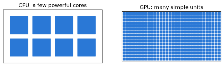
Fig. 3.1 CPU and GPU cores (schematic, not to scale)#
Another type is Google’s tensor processing unit (TPU), a chip designed for the large matrix calculations in machine learning.
Accelerators help only when a task can be split into many similar pieces.
They also have their own memory, so data must be moved onto them before they can work.
3.1.3. Why this matters for AI and statistics#
Training and running a neural network comes down to an enormous number of matrix calculations.
These are exactly the calculations that accelerators are good at, which is why modern AI runs mostly on them.
It is also why the AI tools you use run on a company’s servers rather than on your laptop.
Accelerators matter for statistics too.
For example, the Bayesian analysis that we study in Bayesian Estimation and Uncertainty often relies on running many simulations side by side, which suits a GPU well.
3.1.4. Which library runs on what#
Most policy work runs perfectly well on a laptop CPU, but it helps to know which libraries target which hardware.
Library |
Main use |
Runs on |
|---|---|---|
NumPy, SciPy |
Arrays and scientific routines |
CPU |
pandas |
Tables of data |
CPU |
Matplotlib, seaborn |
Figures |
CPU |
statsmodels |
Statistical models |
CPU |
scikit-learn |
Machine learning |
CPU, with experimental GPU support |
Tables of data |
All CPU cores, with optional NVIDIA GPU support |
|
Tables of data, in the style of pandas |
NVIDIA GPU |
|
Deep learning |
CPU, GPU |
|
Deep learning |
CPU, GPU, TPU |
|
Fast array calculations in the style of NumPy |
CPU, GPU, TPU |
|
Bayesian analysis |
CPU, GPU (built on JAX) |
Google Colab offers access to GPUs and TPUs, and you can try them under Runtime, then Change runtime type.
3.2. NumPy#
NumPy is the foundation of numerical work in Python, and it provides fast operations on arrays and matrices.
3.2.1. Fast array operations#
Here we add up the squares of a million random numbers, first with a Python loop.
rng = np.random.default_rng(1234)
x = rng.uniform(size=1_000_000)
%%time
total = 0
for v in x:
    total = total + v**2
CPU times: user 159 ms, sys: 873 μs, total: 160 ms
Wall time: 160 ms
Now we do the same calculation with NumPy.
%%time
total = np.sum(x**2)
CPU times: user 580 μs, sys: 963 μs, total: 1.54 ms
Wall time: 1.37 ms
Compare the two “Wall time” figures, which show how long each one took.
NumPy is much faster because it passes the work to precompiled code that runs without the overhead of a Python loop.
Operating on a whole array at once like this is called vectorization.
3.2.2. Matrices and linear equations#
Many problems reduce to solving a system of linear equations.
Suppose that demand and supply for a good satisfy \(q = 10 - p\) and \(q = 2 + p\), where \(q\) is quantity and \(p\) is price.
We can rewrite these two equations as
Next we collect the coefficients in a matrix, and the unknowns and the right-hand side in vectors.
This has the form \(A x = b\), and multiplying each row of \(A\) by \(x\) gives back one of the original equations.
NumPy can now solve the system directly.
A = np.array([[1, 1],
              [1, -1]])
b = np.array([10, 2])

np.linalg.solve(A, b)
array([6., 4.])
So the quantity is 6 and the price is 4, which is where the two lines cross.
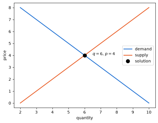
Fig. 3.2 Solving two equations graphically#
The same command works for much larger systems, such as one with 8,000 equations and 8,000 unknowns.
n = 8_000
A = rng.normal(size=(n, n))
b = rng.normal(size=n)
%%time
x = np.linalg.solve(A, b)
CPU times: user 7.31 s, sys: 271 ms, total: 7.58 s
Wall time: 3.79 s
Calculations like this one are the kind of work that accelerators speed up.
JAX lets us run them on an accelerator with almost no change to the code, because jnp is its version of NumPy.
First we ask which hardware JAX can see.
jax.devices()
[CpuDevice(id=0)]
This page was built on a machine with no accelerator, so JAX reports a CPU.
Here is the same calculation in JAX, which we run once as a warm-up.
x = jnp.linalg.solve(A, b).block_until_ready()
The first run is slower, because JAX compiles the calculation for the hardware, so a fair timing needs a second run.
%%time
x = jnp.linalg.solve(A, b).block_until_ready()
CPU times: user 4.19 s, sys: 345 ms, total: 4.54 s
Wall time: 2.28 s
We need block_until_ready because JAX otherwise moves on to the next line while the calculation is still running.
Compare this with the NumPy timing above: at this size, JAX often wins even on a CPU.
On an accelerator, the gap can be far larger: in one test on a desktop GPU, a system of this size took about 0.04 seconds, compared to 0.6 seconds for NumPy on that machine’s CPU.
These comparisons flatter JAX, since it uses lower-precision numbers by default, while NumPy uses higher precision.
To try this yourself, choose a GPU in Colab under Runtime, then Change runtime type, and run these cells again.
3.3. SciPy#
SciPy builds on NumPy, with routines for probability distributions, optimization, numerical integration and more.
As an example, consider finding the area under a curve, which is called numerical integration.
The simplest approach is to cover the area with rectangles and add up their areas, as in the figure below.
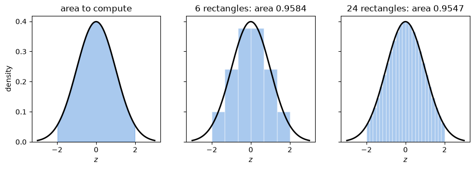
Fig. 3.3 Approximating an area with rectangles#
The approximation improves as the rectangles get narrower.
SciPy’s quad function uses a more sophisticated version of this idea.
Here it computes the same area, under the normal density between \(-2\) and \(2\).
value, error = quad(ϕ.pdf, -2, 2)
value
0.9544997361036417
3.4. Visualizing data#
Python has excellent libraries for visualization, and asking an AI for a figure is one of the best uses of it.
3.4.1. Comparing countries with seaborn#
Seaborn produces statistical figures from a table of data with very little code.
We use the Gapminder data, which contains life expectancy, income and population by country.
gapminder = px.data.gapminder()
gapminder_2007 = gapminder[gapminder['year'] == 2007]
gapminder_2007[['country', 'continent', 'lifeExp', 'pop', 'gdpPercap']].head()
| country | continent | lifeExp | pop | gdpPercap | |
|---|---|---|---|---|---|
| 11 | Afghanistan | Asia | 43.828 | 31889923 | 974.580338 |
| 23 | Albania | Europe | 76.423 | 3600523 | 5937.029526 |
| 35 | Algeria | Africa | 72.301 | 33333216 | 6223.367465 |
| 47 | Angola | Africa | 42.731 | 12420476 | 4797.231267 |
| 59 | Argentina | Americas | 75.320 | 40301927 | 12779.379640 |
The next figure shows how life expectancy rises with income, with a separate panel for each continent and larger dots for larger populations.
g = sns.relplot(data=gapminder_2007, x='gdpPercap', y='lifeExp',
                col='continent', col_wrap=3, height=2.6,
                size='pop', sizes=(10, 400), color=blue, alpha=0.6,
                legend=False, facet_kws={'despine': False})
g.set(xscale='log')
g.set_titles('{col_name}')
g.set_axis_labels('GDP per capita (log scale)', 'life expectancy')
plt.show()
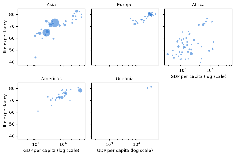
Fig. 3.4 Income and life expectancy, 2007#
A violin plot shows the whole distribution within each group, which a simple average would hide.
Here we leave out Oceania, which has only two countries in these data.
data = gapminder_2007[gapminder_2007['continent'] != 'Oceania']

fig, ax = plt.subplots()
sns.violinplot(data=data, x='continent', y='lifeExp', color=blue,
               inner='quartile', cut=0, density_norm='width', ax=ax)
ax.set_xlabel('continent')
ax.set_ylabel('life expectancy')
plt.show()
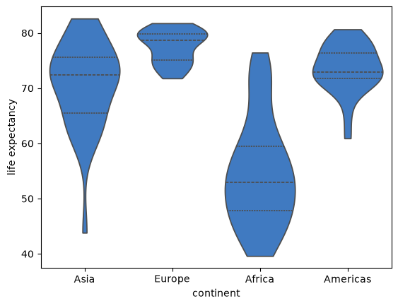
Fig. 3.5 Life expectancy by continent, 2007#
A heat map shows many numbers at once, using color for their size.
table = gapminder.pivot_table(index='continent', columns='year', values='lifeExp')

fig, ax = plt.subplots(figsize=(9, 3.2))
sns.heatmap(table, cmap=blues, annot=True, fmt='.0f', linewidths=1,
            cbar_kws={'label': 'years'}, ax=ax)
ax.set_xlabel('year')
ax.set_ylabel('continent')
plt.show()
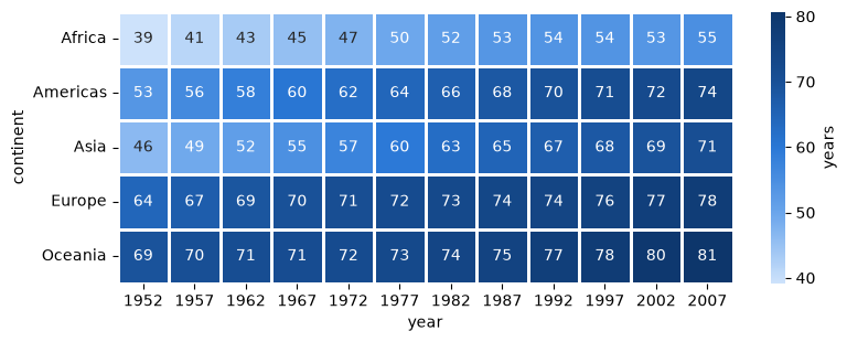
Fig. 3.6 Mean life expectancy by continent and year#
3.4.2. Time series#
A time series records a quantity over time.
Here is life expectancy in four countries from 1952, where the sharp fall for China coincides with the famine of 1959 to 1961.
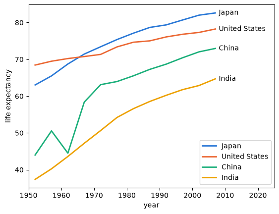
Fig. 3.7 Life expectancy in four countries#
Next is the concentration of carbon dioxide in the atmosphere, measured weekly at Mauna Loa in Hawaii.
The left panel shows the long-run rise, while the right panel zooms in to reveal a seasonal cycle.
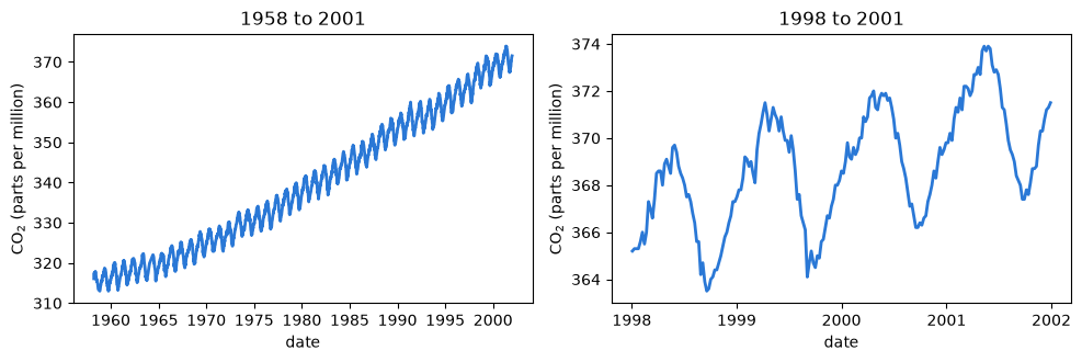
Fig. 3.8 Atmospheric carbon dioxide at Mauna Loa#
3.4.3. Maps#
A choropleth map uses color to show a quantity across regions.
The next figure shows the population of Japan’s 47 prefectures in the 2020 census, using boundaries from Natural Earth.
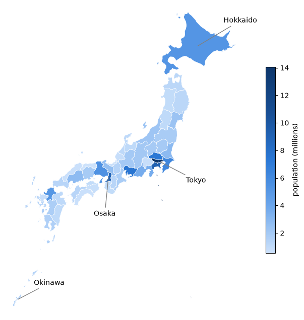
Fig. 3.9 Population of Japan by prefecture, 2020#
The dark region around Tokyo shows how concentrated the population is.
Notice that large prefectures such as Hokkaido look important on a map even when they have relatively few people, which is a common way for maps to mislead.
3.5. Networks#
A network is a set of nodes connected by links, and the NetworkX library works with them in Python.
The next figure shows international trade in large commercial aircraft in 2019, using data from Sargent and Stachurski [2024].
Each node is a country, and each arrow is a flow of exports.
Larger nodes export more, and darker nodes are more central to the network.
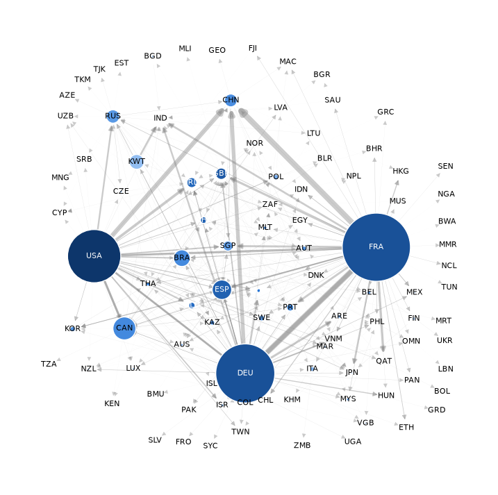
Fig. 3.10 International trade in commercial aircraft, 2019#
Small networks can be just as revealing, and they take very little code.
This one shows marriage ties between leading families in fifteenth-century Florence, a classic example from Padgett and Ansell [1993], and it ships with NetworkX.
We size each family by betweenness centrality, which measures how often it lies on the shortest path between other families.
families = nx.florentine_families_graph()
centrality = nx.betweenness_centrality(families)
sizes = [300 + 6000 * centrality[family] for family in families]

positions = nx.spring_layout(families, seed=1234)

fig, ax = plt.subplots(figsize=(8, 6))
nx.draw_networkx_edges(families, positions, edge_color='gray', ax=ax)
nx.draw_networkx_nodes(families, positions, node_size=sizes,
                       node_color='#9ec5f4', edgecolors=blue, ax=ax)
nx.draw_networkx_labels(families, positions, font_size=9, ax=ax)
ax.axis('off')
plt.show()
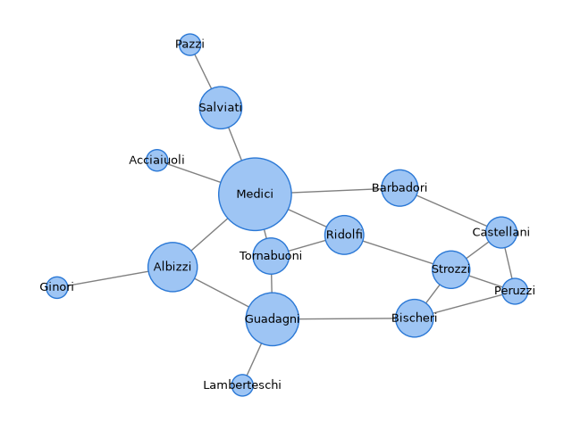
Fig. 3.11 Marriage ties in fifteenth-century Florence#
The Medici stand out as the most central family.
We return to networks in Networks.
3.6. pandas and Polars#
pandas is the standard library for working with tables of data, and we study it in Working with Data.
For example, this line finds the median life expectancy on each continent.
gapminder_2007.groupby('continent')['lifeExp'].median()
continent
Africa      52.9265
Americas    72.8990
Asia        72.3960
Europe      78.6085
Oceania     80.7195
Name: lifeExp, dtype: float64
Polars does a similar job with a different design, and it uses all of your CPU’s cores by default.
It can be much faster on large data sets, but pandas remains the most common choice, and it is what most AI tools produce by default.
3.7. scikit-learn#
scikit-learn is the standard library for machine learning outside of deep learning.
As an example, we ask its k-means algorithm to divide the countries into three groups, using only income and life expectancy.
The algorithm is never told what the groups should be.
features = np.column_stack([np.log(gapminder_2007['gdpPercap']),
                            gapminder_2007['lifeExp'] / 10])

model = KMeans(n_clusters=3, n_init=10, random_state=1234)
labels = model.fit_predict(features)

fig, ax = plt.subplots()

for k, (color, marker) in enumerate(zip([blue, orange, aqua], ['o', 's', '^'])):
    group = gapminder_2007[labels == k]
    ax.scatter(group['gdpPercap'], group['lifeExp'], s=50, color=color,
               marker=marker, edgecolor='white', label=f'cluster {k + 1}')

ax.set_xscale('log')
ax.set_xlabel('GDP per capita (log scale)')
ax.set_ylabel('life expectancy')
ax.legend()
plt.show()
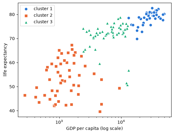
Fig. 3.12 Three clusters of countries, 2007#
The groups look sensible, but the algorithm will always return three groups when asked, whether or not three real groups exist.
Deciding whether they mean anything is your job, as we discuss in Classification, Clustering and Forecasting.
3.8. Git and GitHub#
Finally, we turn to a tool for keeping track of changes to code.
Git is a version control system, which records each saved version of a project, called a commit.
GitHub is a website that stores these projects online, so that people can share them and work on them together.
Most of the libraries above keep their code on GitHub, and so does this book.
Version control matters even more when an AI is editing your work, since it shows you exactly what changed.
This view is called a diff, where red lines were removed and green lines were added.
- if m > 25:
+ if m >= 25:
      count = count + 1
Here an AI has changed > to >=, a small edit that changes the answer, as we saw in Reading Python and Directing AI.
If you do not like a change, then you can go back to the previous commit, which makes it safer to let an AI make large edits.
A branch is a separate line of work within a project, which leaves the main version, usually called main, untouched.
If the work on a branch turns out well, you merge it into main, and if not, you delete the branch and nothing is lost.
The figure below shows both outcomes, where each circle is a commit.
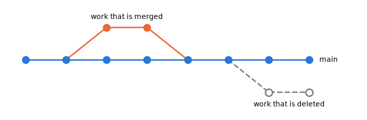
Fig. 3.13 Branching, merging and deleting a branch#
Branches are helpful even when you work alone, particularly with an AI.
For example, you can ask an AI to try a risky change or a new approach on its own branch, and then review the diff before deciding whether to keep it.