6. Observed Distributions and Matching Them to Data#
6.1. Outline#
In Probability Distributions we studied probability distributions, which are one component of probability theory.
In this lecture we turn to observed data — sets of numbers that we measure or collect.
What is the connection between these data and probability distributions?
In this lecture we attempt to answer this question.
Along the way, we discuss how to summarize and visualize such data, and how to determine which probability distribution best describes a given data set.
In addition to what’s in Anaconda, this lecture needs the following library:
!pip install --upgrade yfinance
We use the following imports.
import os

import matplotlib.pyplot as plt
import pandas as pd
import numpy as np
import yfinance as yf
import scipy.stats
import seaborn as sns
We’ll print scalars as plain numbers
np.set_printoptions(legacy='1.25')
6.2. Histograms#
Given a new data set on a single variable, the first thing we usually want to do is look at it.
The standard way is via a histogram, which divides the data into bins and shows how many observations fall in each.
Let’s start with the sale prices of 2,930 houses sold in Ames, Iowa between 2006 and 2010, which come with a few characteristics of each house [De Cock, 2011].
url = ('https://github.com/QuantEcon/data-lectures/raw/main/'
       'lectures/ames_house_prices.csv')
houses = pd.read_csv(url)
price = houses['price']
houses.head()
| price | bedrooms | living_area_sqft | year_built | neighborhood | |
|---|---|---|---|---|---|
| 0 | 215000 | 3 | 1656 | 1960 | NAmes |
| 1 | 105000 | 2 | 896 | 1961 | NAmes |
| 2 | 172000 | 3 | 1329 | 1958 | NAmes |
| 3 | 244000 | 3 | 2110 | 1968 | NAmes |
| 4 | 189900 | 3 | 1629 | 1997 | Gilbert |
Here is a histogram of the sale prices.
fig, ax = plt.subplots()
ax.hist(price, bins=50, density=True)
ax.set_xlabel('sale price (US$)')
ax.set_ylabel('density')
plt.show()
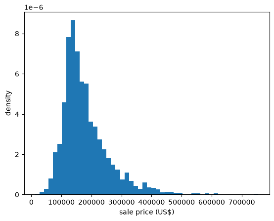
Fig. 6.1 Histogram of house prices#
The data have a long right tail: a small number of houses sell for far more than the typical price.
Data like this often look more symmetric after taking logarithms.
log_price = np.log(price)

fig, ax = plt.subplots()
ax.hist(log_price, bins=50, density=True)
ax.set_xlabel('log of sale price')
ax.set_ylabel('density')
plt.show()
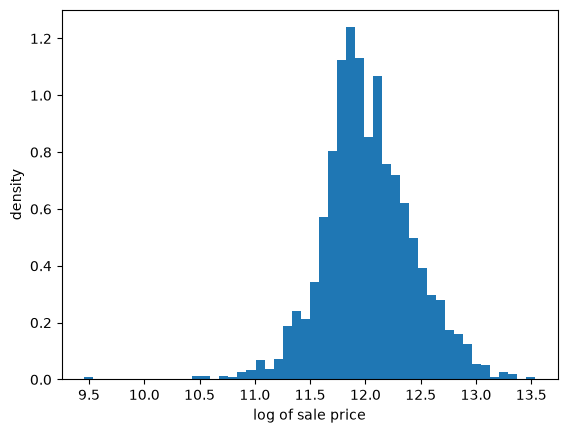
Fig. 6.2 Histogram of log house prices#
This histogram is far more symmetric.
For a second example, let’s look at the GDP of each country in 2025, in US dollars, from the World Bank.
path = '_static/lecture_specific/observed_distributions/gdp_by_country_2025.csv'
url = ('https://raw.githubusercontent.com/jstac/py_for_ds_public/main/lectures/'
       + path)

# use the copy stored with this book if there is one, and otherwise download it
gdp = pd.read_csv(path if os.path.exists(path) else url)
gdp.head()
| country | code | gdp_usd | |
|---|---|---|---|
| 0 | Albania | ALB | 3.054019e+10 |
| 1 | Algeria | DZA | 2.870312e+11 |
| 2 | Andorra | AND | 4.500983e+09 |
| 3 | Angola | AGO | 1.221749e+11 |
| 4 | Antigua and Barbuda | ATG | 2.338196e+09 |
Here are histograms of GDP and of its logarithm, showing the number of countries in each bin.
We use base 10 logarithms, so each unit on the horizontal axis of the right-hand panel is a factor of ten.
log_gdp = np.log10(gdp['gdp_usd'])

fig, axes = plt.subplots(1, 2, figsize=(10, 4))
axes[0].hist(gdp['gdp_usd'] / 1e12, bins=50)
axes[0].set_xlabel('GDP (trillions of US$)')
axes[0].set_ylabel('number of countries')
axes[1].hist(log_gdp, bins=25)
axes[1].set_xlabel('log10 of GDP (US$)')
plt.show()
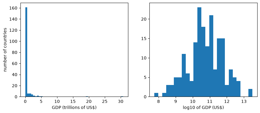
Fig. 6.3 GDP by country, 2025#
The United States and China, at about 31 and 20 trillion dollars, are so much larger than the rest that they stretch the horizontal axis, and 161 of the 186 countries fall in the first bin.
The right tail is even longer than for house prices.
On a log scale, the distribution is close to symmetric.
6.3. Sample moments and quantiles#
Histograms show us the shape of a data set, and we often want to summarize that shape with a few numbers as well.
We start with sample moments, which are averages of powers of the data, and then turn to sample quantiles.
6.3.1. Sample mean and variance#
Suppose we have a data set with values \(\{x_1, \ldots, x_n\}\).
The sample mean of this distribution is defined as
The sample variance is defined as
and the sample standard deviation \(s\) is its square root.
For example, suppose that we observe the income of 10 people during one year:
data = [['Hiroshi', 1200],
        ['Ako', 1210],
        ['Emi', 1400],
        ['Daiki', 990],
        ['Chiyo', 1530],
        ['Taka', 1210],
        ['Katsuhiko', 1240],
        ['Daisuke', 1124],
        ['Yoshi', 1330],
        ['Rie', 1340]]

df = pd.DataFrame(data, columns=['name', 'income'])
df
| name | income | |
|---|---|---|
| 0 | Hiroshi | 1200 |
| 1 | Ako | 1210 |
| 2 | Emi | 1400 |
| 3 | Daiki | 990 |
| 4 | Chiyo | 1530 |
| 5 | Taka | 1210 |
| 6 | Katsuhiko | 1240 |
| 7 | Daisuke | 1124 |
| 8 | Yoshi | 1330 |
| 9 | Rie | 1340 |
Here we compute the sample mean and sample variance, as well as the sample standard deviation.
income = df['income']
income.mean(), income.var(ddof=0), income.std(ddof=0)
(1257.4, 20412.839999999997, 142.8735104909234)
Note
By default, pandas divides by \(n-1\) rather than \(n\) when computing the variance and standard deviation.
Setting ddof=0 makes it divide by \(n\), as in the formula above.
The difference is small when \(n\) is large.
Notice that these sample moments have a clear connection to the population moments defined in Probability Distributions.
They are the mean, variance, and standard deviation of a finite probability distribution that puts equal probability \(1/n\) on each observed outcome \(x_i\).
The sample moments discussed below also follow this pattern.
6.3.2. Higher sample moments#
The sample skewness and sample kurtosis are
The sample excess kurtosis is \(\hat K - 3\).
Recall from Probability Distributions that a normal distribution has skewness zero and excess kurtosis zero.
This gives us one way to ask whether a data set looks normal.
Let’s try it on the heights of US adult women, which we saw in Fig. 5.2 were well described by a normal distribution.
Note
scipy.stats.kurtosis returns the excess kurtosis.
url = ('https://github.com/QuantEcon/data-lectures/raw/main/'
       'lectures/us_adult_heights.csv')
heights = pd.read_csv(url)
female = heights[heights['sex'] == 'female']['height_cm']

scipy.stats.skew(female), scipy.stats.kurtosis(female)
(0.06940271585060076, -0.009473050923347603)
Both numbers are close to zero, which is consistent with the histograms in Probability Distributions.
Now let’s compute the same statistics for the house prices.
scipy.stats.skew(price), scipy.stats.kurtosis(price)
(1.7426073719460107, 5.108121716933333)
The skewness is large and positive, which is how it registers the long right tail we saw in the histogram.
The excess kurtosis is also large, telling us that extreme values are much more common than they would be for a normal distribution.
We saw exactly this combination in Probability Distributions when we looked at the lognormal distribution.
For the log prices, the numbers match the more symmetric histogram.
scipy.stats.skew(log_price), scipy.stats.kurtosis(log_price)
(-0.014785864999287298, 1.509277466509812)
The skewness is now almost exactly zero.
In other words, the logarithm of the sale price looks far more symmetric than the sale price itself, as it would if prices were lognormal.
The GDP data are more extreme still, with skewness close to zero only after taking logs.
scipy.stats.skew(gdp['gdp_usd']), scipy.stats.skew(log_gdp)
(8.968267093898803, -0.14573616522286542)
Our last example runs in the opposite direction.
The next cell reads the number of deaths in Japan in 2023 at each single year of age, from the World Population Prospects of the United Nations.
url = ('https://github.com/QuantEcon/data-lectures/raw/main/'
       'lectures/japan_deaths_by_age.csv')
deaths = pd.read_csv(url)
deaths.tail()
| age | deaths_male | deaths_female | deaths_total | |
|---|---|---|---|---|
| 96 | 96 | 9818 | 25563 | 35381 |
| 97 | 97 | 7652 | 22605 | 30258 |
| 98 | 98 | 5757 | 19343 | 25100 |
| 99 | 99 | 4197 | 15801 | 19998 |
| 100 | 100 | 8006 | 42277 | 50284 |
Since the data are counts at each age, a bar chart shows the distribution directly.
fig, ax = plt.subplots()
ax.bar(deaths['age'], deaths['deaths_total'] / 1000)
ax.set_xlabel('age at death')
ax.set_ylabel('deaths (thousands)')
plt.show()
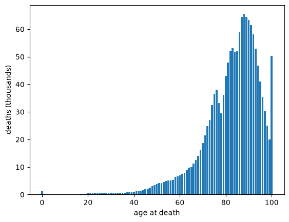
Fig. 6.4 Deaths in Japan by age, 2023#
Deaths cluster at high ages, with a long tail running down towards zero — the mirror image of the house price data.
The last bar is taller than its neighbors because it is recorded as “100 and over”, so it counts every death above age 100, not just deaths at age 100.
Checking for artifacts like this is an important part of looking at data.
To compute statistics, we first expand the counts into a data set with one observation per death.
age_at_death = np.repeat(deaths['age'], deaths['deaths_total'])
len(age_at_death)
1524431
scipy.stats.skew(age_at_death), scipy.stats.kurtosis(age_at_death)
(-1.5993074774223388, 4.579170087851459)
Now the skewness is large and negative, matching the long left tail in the bar chart.
6.3.3. Sample quantiles#
Not every useful summary statistic is a moment.
If we sort the observations from smallest to largest, then the sample \(\tau\)-quantile is the value below which a fraction \(\tau\) of the observations fall.
The 0.5 quantile is the sample median and the 0.25 and 0.75 quantiles are the first and third sample quartiles.
Here are these values for the income data:
income.median(), income.quantile(0.25), income.quantile(0.75)
(1225.0, 1202.5, 1337.5)
Sample quantiles are useful because they are barely affected by a small number of extreme observations.
To see this, let’s replace the largest income in our data set with a very large value and recompute the mean and the median.
income_outlier = income.copy()
income_outlier.iloc[income.argmax()] = 10_000_000

income.mean(), income_outlier.mean()
(1257.4, 1001104.4)
income.median(), income_outlier.median()
(1225.0, 1225.0)
The mean shifts enormously while the median does not move at all.
The same issue arises with real data whenever the distribution is skewed.
Here are the mean and the median sale price of houses in Ames:
price.mean(), price.median()
(180796.0600682594, 160000.0)
The mean exceeds the median by around 13%, pulled up by the expensive houses in the right tail.
This is why house prices are almost always reported as medians.
For the age at death data the inequality runs the other way.
age_at_death.mean(), age_at_death.median()
(82.49081591754563, 85.0)
Here the mean is pulled below the median, by deaths at young ages.
In general, the mean sits on the side of the median towards which the data are skewed.
The gap can be far larger for wealth, which has a very long right tail.
The next cell reads the net worth of US households in 2022, from the Federal Reserve’s Survey of Consumer Finances.
url = ('https://github.com/QuantEcon/data-lectures/raw/main/'
       'lectures/us_household_net_worth_2022.csv')
wealth = pd.read_csv(url)
wealth.head()
| yy1 | y1 | wgt | networth | |
|---|---|---|---|---|
| 0 | 1 | 11 | 3027.956120 | 762100.0 |
| 1 | 1 | 12 | 3054.900065 | 854300.0 |
| 2 | 1 | 13 | 3163.637766 | 678200.0 |
| 3 | 1 | 14 | 3166.228463 | 279600.0 |
| 4 | 1 | 15 | 3235.624715 | 602600.0 |
The survey deliberately includes extra wealthy households, since a random sample would contain very few of them.
To compensate, each row has a weight wgt, which is the number of US households that the row represents, and we use these weights when computing statistics.
def weighted_median(values, weights):
    "The value at which the sorted weights first reach half of their total."
    order = np.argsort(values)
    cumulative = np.cumsum(weights[order])
    return values[order][np.searchsorted(cumulative, cumulative[-1] / 2)]

net_worth = wealth['networth'].to_numpy()
weights = wealth['wgt'].to_numpy()

mean_wealth = np.average(net_worth, weights=weights)
median_wealth = weighted_median(net_worth, weights)

mean_wealth, median_wealth
(1059457.4704505308, 192700.0)
Mean wealth is more than five times median wealth.
So the “average” household is much wealthier than a typical one, and a policy discussion needs to be clear about which it means.
The true gap is a little larger still, because the survey leaves out the very richest households, such as the Forbes 400, a point we return to in Application: A Wealth Tax.
Similar gaps appear across countries, as this ranking by average and median wealth shows.
6.4. More ways to visualize data#
Histograms are not the only way to look at a data set.
Here are four more, each suited to a different purpose.
6.4.1. Empirical cumulative distribution functions#
A histogram estimates the density of the data.
The empirical cumulative distribution function (ECDF) does the same job for the CDF.
For a sample \(\{x_1, \ldots, x_n\}\) it is defined as
In words, \(F_n(x)\) is just the fraction of observations that are less than or equal to \(x\).
The ECDF is a step function that jumps up by \(1/n\) at each observation.
Here is a function that plots it, obtained by sorting the data and stepping up as we move from left to right.
def plot_ecdf(sample, ax, **kwargs):
    x_sorted = np.sort(sample)
    n = len(x_sorted)
    ax.step(x_sorted, np.arange(1, n+1) / n, where='post', **kwargs)
Unlike a histogram, the ECDF requires no choice of bin width — it uses the data exactly as they are.
This makes it a good tool for comparing a data set with a probability distribution, since we can simply plot the two curves on the same axes.
Let’s compare the log prices with the CDF of the normal distribution that has the same mean and standard deviation.
u = scipy.stats.norm(log_price.mean(), log_price.std())
x_grid = np.linspace(log_price.min(), log_price.max(), 200)

fig, ax = plt.subplots()
plot_ecdf(log_price, ax, lw=2, label='ECDF of log prices')
ax.plot(x_grid, u.cdf(x_grid), 'k--', alpha=0.7, lw=2, label='normal CDF')
ax.set_xlabel('log of sale price')
ax.set_ylabel('probability')
ax.legend()
plt.show()
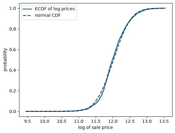
Fig. 6.5 Log prices against a normal CDF#
The two curves are close, although the fit is not perfect.
6.4.2. Kernel density estimates#
A histogram depends on where we place the bins, and its blocky shape comes from the bins rather than the data.
A kernel density estimate (KDE) avoids both problems.
Instead of adding a block to a bin, it adds a small smooth bump, called a kernel, centered on each observation.
The estimate is the sum of these bumps, rescaled so that it integrates to one:
Here \(K\) is the kernel, usually a normal density, and the bandwidth \(h\) sets the width of each bump.
The next figure shows both methods at work on six observations, which are marked along the horizontal axis.
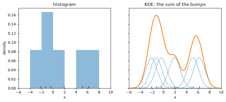
Fig. 6.6 A histogram and a KDE of the same six observations#
The KDE has no bins, but it does have a choice to make: the bandwidth.
Let’s look at the log sale price data at three bandwidths, using the kdeplot function from Seaborn, where bw_adjust scales its default choice.
fig, ax = plt.subplots()
for bw in (0.1, 0.5, 2):
    sns.kdeplot(log_price, ax=ax, bw_adjust=bw, lw=2, label=f'bw_adjust={bw}')
ax.set_xlabel('log of sale price')
ax.set_ylabel('density')
ax.legend()
plt.show()
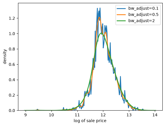
Fig. 6.7 KDE of log prices at three bandwidths#
A larger bandwidth gives a smoother curve.
A suitable bandwidth is neither too wiggly, chasing individual observations, nor too smooth, hiding real features of the data.
Since a KDE is a smoothed histogram, it is often helpful to show the two together.
fig, ax = plt.subplots()
ax.hist(log_price, bins=50, density=True, alpha=0.25, color='C0')
sns.kdeplot(log_price, ax=ax, color='C0', lw=2)
ax.set_xlabel('log of sale price')
ax.set_ylabel('density')
plt.show()
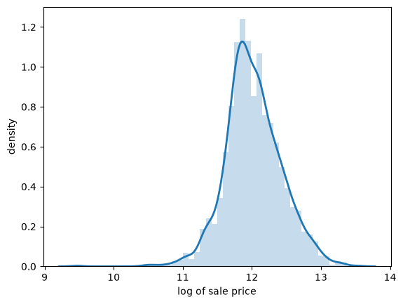
Fig. 6.8 KDE and histogram of log prices#
The KDE traces out the shape of the histogram while smoothing away the bin-to-bin variation.
6.4.3. Box-and-whisker plots#
A box-and-whisker plot (or box plot) summarizes a distribution using the sample quantiles discussed above.
The box spans the first and third quartiles, and the line inside it is the median.
The whiskers extend to the most extreme observations lying within 1.5 times the height of the box, and observations beyond them are plotted individually.
Box plots discard a lot of information, which makes them well suited to comparing many groups at once.
For example, let’s compare house prices across houses with different numbers of bedrooms.
bedroom_counts = (1, 2, 3, 4, 5)
groups = [price[houses['bedrooms'] == b] for b in bedroom_counts]

fig, ax = plt.subplots()
ax.boxplot(groups, tick_labels=bedroom_counts)
ax.set_xlabel('bedrooms')
ax.set_ylabel('sale price (US$)')
plt.show()
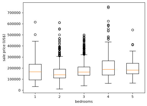
Fig. 6.9 House prices by number of bedrooms#
The figure carries a warning about reading too much into group averages.
Houses with four bedrooms do sell for more than houses with three, but one-bedroom houses have a higher median price than two-bedroom houses.
Moreover, the spread within every group is far larger than the differences across groups.
Evidently the number of bedrooms tells us relatively little about the price of a house.
6.4.4. Violin plots#
A violin plot shows a KDE on each side of a vertical line, which makes it easy to compare the shapes of several distributions.
Let’s return to the age at death data and separate men from women.
male_deaths = np.repeat(deaths['age'], deaths['deaths_male'])
female_deaths = np.repeat(deaths['age'], deaths['deaths_female'])

fig, ax = plt.subplots()
ax.violinplot([male_deaths, female_deaths], showmedians=True)
ax.set_ylabel('age at death')
ax.set_xlabel('sex')

ax.set_xticks([1, 2])
ax.set_xticklabels(['male', 'female'])
plt.show()
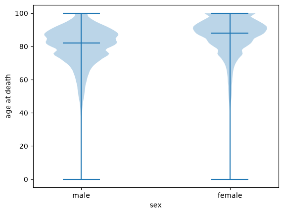
Fig. 6.10 Age at death, male and female#
The violin plot shows the whole shape of each distribution, rather than the five numbers that a box plot reduces it to.
Here that matters: both distributions are strongly left-skewed, with a thin tail of deaths at young ages, and the female distribution is shifted upwards, with a median of 88 against 82 for men.
6.5. Why samples tell us about distributions#
Let’s now discuss the connection between observed distributions and probability distributions.
It is often helpful to imagine that an observed distribution was generated by a particular probability distribution.
Throughout this lecture we have used observed data to say something about such an underlying distribution.
This only works if a larger sample tells us more.
6.5.1. Larger samples#
Let’s check that it does, using the ECDF, since it estimates the CDF without requiring us to choose a bin width or a bandwidth.
We draw samples of increasing size from a fixed distribution and compare each ECDF with the CDF that generated it.
u = scipy.stats.lognorm(s=0.5)
x_grid = np.linspace(0, 5, 200)

fig, ax = plt.subplots()
for n in (10, 100, 1000):
    x_draws = u.rvs(n, random_state=1234)
    plot_ecdf(x_draws, ax, alpha=0.7, lw=2, label=f'$n = {n}$')
ax.plot(x_grid, u.cdf(x_grid), 'k--', lw=2, label='true CDF')
ax.set_xlabel('x')
ax.set_ylabel('probability')
ax.legend()
plt.show()
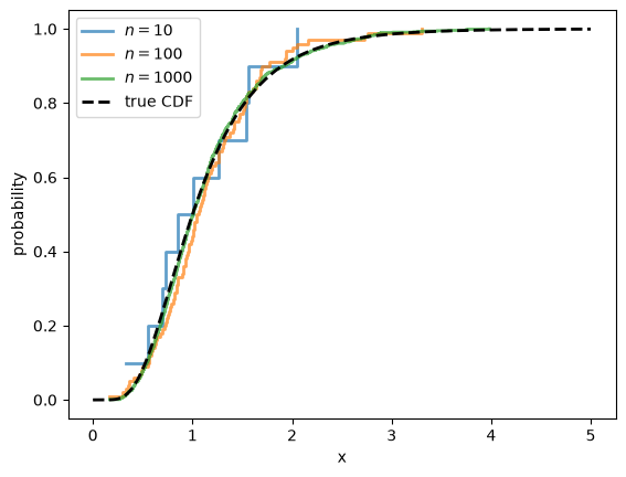
Fig. 6.11 ECDFs converge to the true CDF#
The ECDF is ragged when \(n = 10\) and almost indistinguishable from the true CDF by the time \(n = 1000\).
The sample mean behaves the same way.
for n in (10, 100, 1000, 1_000_000):
    x_draws = u.rvs(n, random_state=1234)
    print(f'n = {n:>9,}:  sample mean = {x_draws.mean():.4f}')
print(f'{"":16}population mean = {u.mean():.4f}')
n =        10:  sample mean = 1.0573
n =       100:  sample mean = 1.1398
n =     1,000:  sample mean = 1.1340
n = 1,000,000:  sample mean = 1.1332
                population mean = 1.1331
6.5.2. The law of large numbers#
These results are examples of the law of large numbers (LLN).
It says that, if \(X_1, \ldots, X_n\) are independent draws from a distribution with finite mean \(\mu\), then
with probability one.
The same result applies to the average of any function \(f(X_i)\), provided that \(\mathbb{E}[f(X_i)]\) is finite.
Taking \(f(x) = x^k\) shows why sample moments recover population moments.
Taking \(f(x_i) = \mathbb 1\{x_i \leq x\}\) shows why the ECDF converges to the CDF, since \(F_n(x)\) is just the average of these indicators.
So the LLN is the basic reason that data can teach us about distributions.
It has two conditions, independence and a finite mean, and we consider each in turn.
6.5.3. The role of independence#
The convergence above is not automatic.
It depends on a property of the sample that is easy to overlook, because rvs supplies it silently: the draws it returns are independent.
To see why this matters, suppose we take a single draw \(X\) from our distribution and then set
Every \(X_i\) now has exactly the right distribution.
Judged one at a time, these are perfectly good observations.
But they are useless as a sample, as the next figure shows.
x_single = u.rvs(random_state=1234)         # a single draw

fig, ax = plt.subplots()
for n in (10, 100, 1000):
    x_draws = np.full(n, x_single)          # repeated n times
    plot_ecdf(x_draws, ax, alpha=0.7, lw=2, label=f'$n = {n}$')
ax.plot(x_grid, u.cdf(x_grid), 'k--', lw=2, label='true CDF')
ax.set_xlabel('x')
ax.set_ylabel('probability')
ax.legend()
plt.show()
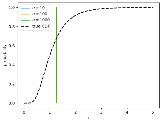
Fig. 6.12 Repeated draws of a single value#
The three ECDFs lie exactly on top of one another: each is a single step at \(X\), and increasing \(n\) changes nothing.
The sample never approaches the distribution it came from, no matter how large we make it.
The reason is that the observations after the first one carry no information we did not already have.
Note
Independence is a clean sufficient condition rather than a necessary one.
Many dependent samples work perfectly well, as we see in Markov Chains and Social Mobility.
What matters is that new observations keep bringing new information, which the example above destroys entirely.
6.6. When sample means fail#
The second condition for the LLN is a finite mean.
This matters because, as we saw in Probability Distributions, heavy-tailed distributions can have infinite moments.
Let’s run a simulation with three distributions, each sampled independently:
an exponential distribution with mean 3
a Pareto distribution with tail index 1.5, which also has mean 3 but has infinite variance
a Pareto distribution with tail index 1, which has infinite mean
For each one, we plot how the sample mean evolves as the sample grows, for five separate runs.
rng = np.random.default_rng(1234)
n = 100_000
sample_sizes = np.arange(1, n+1)

cases = (('exponential, mean 3', scipy.stats.expon(scale=3), 3),
         ('Pareto, tail index 1.5, mean 3', scipy.stats.pareto(1.5), 3),
         ('Pareto, tail index 1, infinite mean', scipy.stats.pareto(1), None))

fig, axes = plt.subplots(3, 1, sharex=True, figsize=(8, 9))
for ax, (title, u, mean) in zip(axes, cases):
    for run in range(5):
        draws = u.rvs(n, random_state=rng)
        ax.plot(sample_sizes, np.cumsum(draws) / sample_sizes, lw=2, alpha=0.7)
    if mean is not None:
        ax.axhline(mean, color='k', ls='--', lw=2)
    else:
        ax.set_yscale('log')
    ax.set_xscale('log')
    ax.set_title(title)
    ax.set_ylabel('sample mean')
axes[-1].set_xlabel('sample size')
plt.tight_layout()
plt.show()
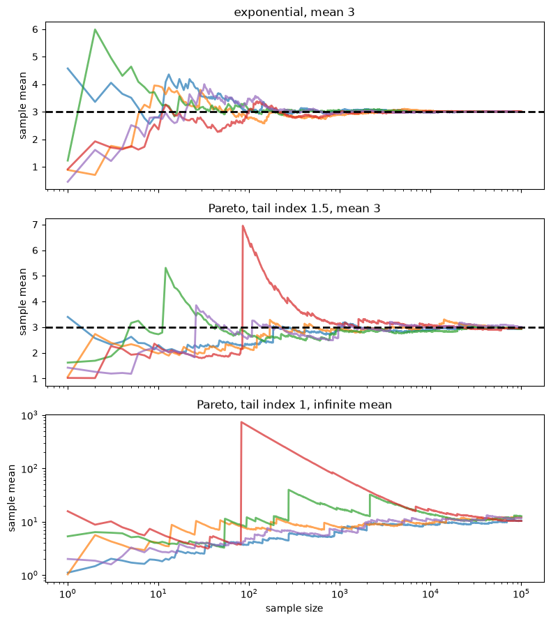
Fig. 6.13 The sample mean as the sample grows#
The exponential sample means settle down quickly at the population mean, shown by the dashed line.
The sample means for the Pareto with tail index 1.5 still converge, as the LLN promises, but slowly and in jumps, each caused by a single huge observation.
With tail index 1 the LLN does not apply, and the sample mean never settles down: it tends to drift upwards, with occasional huge jumps, so this panel uses a logarithmic vertical scale.
The median, by contrast, is well behaved even in this last case, where its population value is 2.
u = scipy.stats.pareto(1)

for n in (100, 10_000, 1_000_000):
    draws = u.rvs(n, random_state=rng)
    print(f'n = {n:>9,}:  mean = {draws.mean():8.2f},  '
          f'median = {np.median(draws):.2f}')
n =       100:  mean =     4.45,  median = 1.78
n =    10,000:  mean =    10.48,  median = 2.00
n = 1,000,000:  mean =    42.49,  median = 2.00
So, with heavy-tailed data, a sample mean can be unreliable even in a large sample.
This is one more reason to look at medians and other quantiles for data such as wealth.
We return to this point in Heavy Tails and Inequality.
6.7. Fitting a distribution#
We now turn to a question that arises constantly in applied work:
given a data set, which probability distribution should we use to describe it?
The question has two parts.
First, we must choose a parametric class — a set of distributions indexed by a small number of parameters.
For example, the normal distributions form a parametric class, indexed by the mean \(\mu\) and the standard deviation \(\sigma\).
Second, having chosen a class, we must choose the parameters within it that make the fit as close as possible.
We start with the parameters, since we have to be able to fit a class before we can judge it.
6.7.1. The method of moments#
One simple and general strategy is the method of moments.
If the class has \(k\) parameters, we
compute the first \(k\) sample moments of the data,
write down the corresponding population moments as functions of the parameters, and
choose the parameters that make the two sets of numbers equal.
In effect we are asking the distribution to reproduce the features of the data that we consider most important.
We have already used this idea once, in Probability Distributions, when we fitted a normal distribution to the heights of US adults.
The normal distribution has two parameters, so we used two moments: we set \(\mu\) equal to the sample mean and \(\sigma\) equal to the sample standard deviation.
Let’s apply the same idea to the house price data, using two classes that live on \((0, \infty)\) and hence respect the fact that prices are positive.
The lognormal distribution has parameters \(\mu\) and \(\sigma\), with
Setting these equal to the sample mean \(\bar x\) and sample variance \(s^2\) and solving gives
The gamma distribution has parameters \(\alpha\) and \(\beta\), with mean \(\alpha / \beta\) and variance \(\alpha / \beta^2\).
Solving in the same way is easier here:
Let’s implement all three fits.
def fit_normal(sample):
    return scipy.stats.norm(sample.mean(), sample.std())

def fit_lognormal(sample):
    m, v = sample.mean(), sample.var()
    σ_squared = np.log(1 + v / m**2)
    μ = np.log(m) - σ_squared / 2
    return scipy.stats.lognorm(s=np.sqrt(σ_squared), scale=np.exp(μ))

def fit_gamma(sample):
    m, v = sample.mean(), sample.var()
    return scipy.stats.gamma(a=m**2 / v, scale=v / m)
Each function returns a distribution object of the kind we worked with in Probability Distributions.
Let’s check that the fitted lognormal reproduces the mean of the data, as it was constructed to do.
u = fit_lognormal(price)
u.mean(), price.mean()
(180796.06006825934, 180796.0600682594)
Now let’s plot the three fitted densities against a histogram of the data.
fits = {'normal': fit_normal(price),
        'lognormal': fit_lognormal(price),
        'gamma': fit_gamma(price)}

x_grid = np.linspace(0, price.max(), 400)

fig, ax = plt.subplots()
ax.hist(price, bins=50, density=True, alpha=0.25, color='C0')
for label, u in fits.items():
    ax.plot(x_grid, u.pdf(x_grid), lw=2, alpha=0.8, label=label)
ax.set_xlabel('sale price (US$)')
ax.set_ylabel('density')
ax.legend()
plt.show()
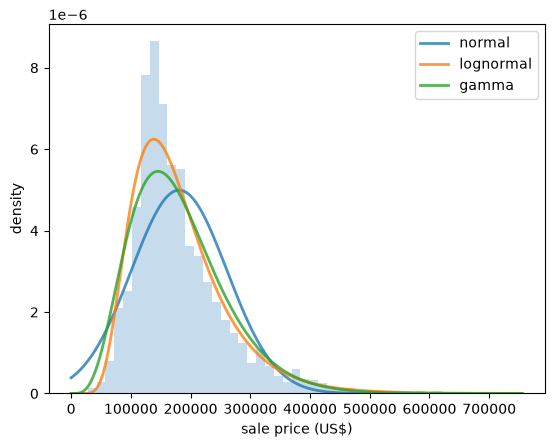
Fig. 6.14 Three fitted densities for house prices#
The normal density is visibly wrong: it is symmetric, while the data are not, and it puts weight on negative prices.
The other two look plausible.
To choose between them we need something sharper than a glance at a figure.
6.7.2. Q-Q plots#
A Q-Q plot (short for quantile-quantile plot) compares two distributions by plotting their quantiles against each other.
To compare a sample with a fitted distribution, we sort the data
We treat \(x_{(i)}\) as an estimate of the quantile of order \((i - 0.5)/n\), since it has about that fraction of the observations below it.
If the fitted distribution is a good description of the data, then \(x_{(i)}\) should be close to the corresponding quantile of that distribution, which is
So we plot the fitted quantiles on the horizontal axis and the sample values on the vertical axis.
A good fit puts the points on the 45 degree line.
def qq_plot(sample, u, ax, **kwargs):
    "Plot sample quantiles against the quantiles of the distribution u."
    x_sorted = np.sort(sample)
    n = len(x_sorted)
    p = (np.arange(1, n+1) - 0.5) / n
    ax.plot(u.ppf(p), x_sorted, '.', ms=3, alpha=0.6, **kwargs)
    lo, hi = u.ppf(p[0]), u.ppf(p[-1])
    ax.plot([lo, hi], [lo, hi], 'k--', lw=2)
    ax.set_xlabel('fitted quantiles')
    ax.set_ylabel('sample quantiles')
Let’s start with a case where we expect a good fit: the heights of US adult women.
fig, ax = plt.subplots()
qq_plot(female, fit_normal(female), ax)
plt.show()
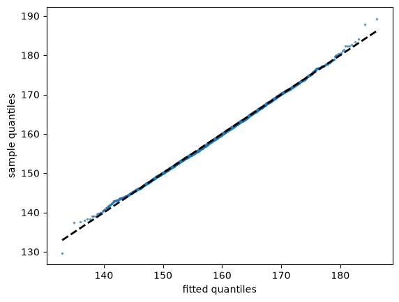
Fig. 6.15 Female heights against a fitted normal#
The points lie almost exactly on the line, apart from mild wandering at the two ends, where the sample contains few observations and the quantile estimates are noisy.
Now let’s try the log house prices.
fig, ax = plt.subplots()
qq_plot(log_price, fit_normal(log_price), ax)
plt.show()
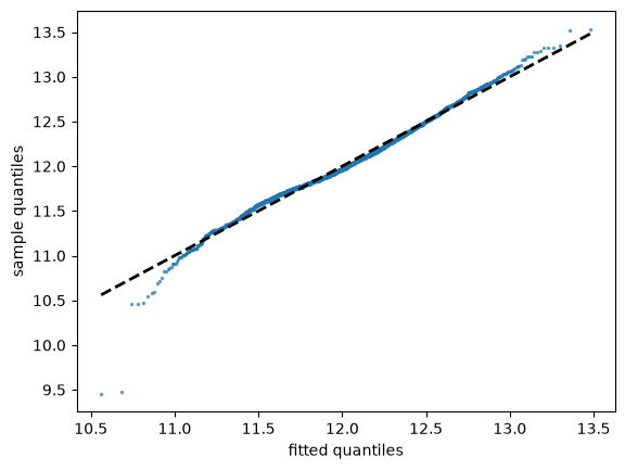
Fig. 6.16 Log house prices against a fitted normal#
The points lie close to the line through most of the distribution, confirming what the sample skewness told us.
The main departure is at the bottom, where a few very cheap houses sold for less than the fitted normal predicts.
6.7.3. Choosing a parametric class#
We can now compare candidate classes by fitting each one and looking at its Q-Q plot.
fig, axes = plt.subplots(1, 3, sharey=True, figsize=(12, 4))
for ax, (label, u) in zip(axes, fits.items()):
    qq_plot(price, u, ax)
    ax.set_title(label)
    ax.tick_params(axis='x', rotation=30)
for ax in axes[1:]:
    ax.set_ylabel('')
plt.tight_layout()
plt.show()
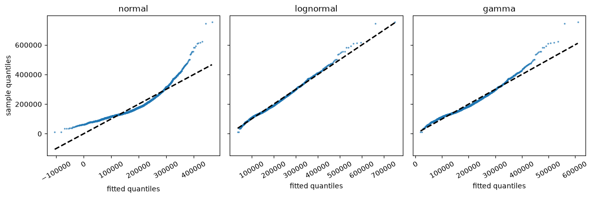
Fig. 6.17 House prices against three fitted classes#
The shape of a departure tells us how a fit fails.
In the normal panel the points curve upwards: towards the right, the sample quantiles are far larger than the fitted ones, so the data have a longer right tail than the normal distribution allows.
The gamma does better, but its points still rise above the line at the top, so its right tail is too short.
The lognormal comes closest, with the points near the line almost everywhere.
This agrees with what we found earlier, where taking logs of the prices produced a sample skewness of almost zero.
Three warnings are in order.
First, such a comparison is only fair when the classes have the same number of parameters, as they do here, since a class with more parameters can bend itself closer to any data set.
Second, a plot like this can show that one class does better in the tails while another does better in the middle, so the choice depends on what we care about.
Third, the winner is only the best of the candidates we happened to try.
Nothing here tells us that the winning class is a good description of the data — only that it is better than the alternatives.
6.7.4. When the normal fails#
Let’s see what a failure of the normal distribution looks like in a case where the data take both signs, so that classes on \((0, \infty)\) are not available.
We look at the monthly return on Amazon shares between 2000 and 2024, measured as the percent change in the share price over each month.
data = yf.download('AMZN', '2000-1-1', '2024-1-1', interval='1mo')
prices = data['Close']['AMZN']
returns = prices.pct_change().dropna() * 100
Here is a histogram of the returns, along with a fitted normal density.
u = fit_normal(returns)
x_grid = np.linspace(returns.min(), returns.max(), 200)

fig, ax = plt.subplots()
ax.hist(returns, density=True, bins=40, alpha=0.5)
ax.plot(x_grid, u.pdf(x_grid), lw=2)
ax.set_xlabel('monthly return (percent change)')
ax.set_ylabel('density')
plt.show()
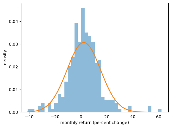
Fig. 6.18 Amazon returns and a fitted normal#
The match is not bad but also not very good.
The Q-Q plot shows what is going on.
fig, ax = plt.subplots()
qq_plot(returns, u, ax)
plt.show()
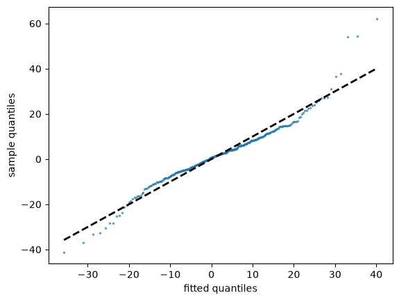
Fig. 6.19 Amazon returns against a fitted normal#
The points form an S-shape: the smallest returns are more negative than the fitted normal predicts, and the largest are more positive.
In other words, both tails of the data are heavier than the normal distribution allows.
The failure is in the tails, and the tails are precisely what a study of asset returns cares about, since they contain the large losses.
The Q-Q plot also suggests a remedy, which is to try a class with heavier tails, as we do in Maximum Likelihood Estimation.
6.8. Exercises#
Exercise 6.1
You ask an AI tool to report typical household wealth in the United States, using the Survey of Consumer Finances data above, and it returns the code below.
print(wealth['networth'].mean())
print(wealth['networth'].median())
The code runs without an error.
What is wrong with the answer?
Run the code and compare its output with the numbers we found in the lecture.
Solution
print(wealth['networth'].mean(), mean_wealth)
print(wealth['networth'].median(), median_wealth)
19956403.324635472 1059457.4704505308
384500.0 192700.0
The code ignores the survey weights.
The survey deliberately includes many wealthy households, so treating each row as equally important overstates wealth.
The unweighted mean is about 19 times the weighted mean, and the unweighted median is about twice the weighted median.
Exercise 6.2
The house price data set also records the floor area of each house, in square feet, in the column living_area_sqft.
Split the houses into four groups of equal size according to floor area (the pandas function qcut will do this for you) and produce a box plot of sale price for each group.
Is floor area a better predictor of price than the number of bedrooms?
Solution
Here is one solution:
area_quartile = pd.qcut(houses['living_area_sqft'], 4,
                        labels=['Q1', 'Q2', 'Q3', 'Q4'])
groups = [price[area_quartile == q] for q in ('Q1', 'Q2', 'Q3', 'Q4')]

fig, ax = plt.subplots()
ax.boxplot(groups, tick_labels=['Q1', 'Q2', 'Q3', 'Q4'])
ax.set_xlabel('quartile of floor area')
ax.set_ylabel('sale price (US$)')
plt.show()
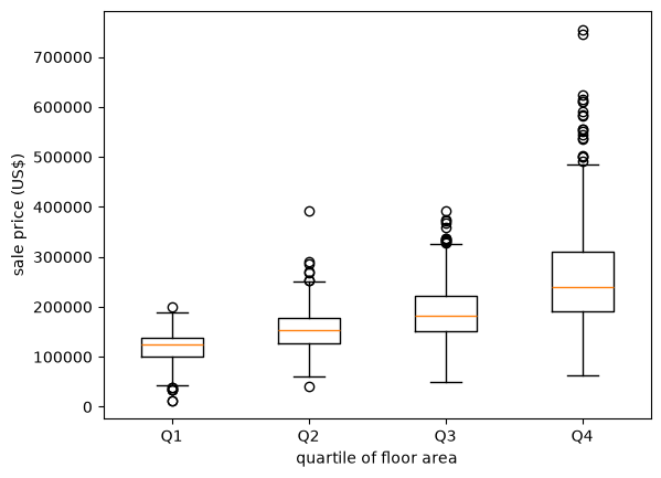
Now the medians increase steadily from one group to the next, and the gaps between the groups are large relative to the spread within them.
Floor area is clearly the better predictor.
Exercise 6.3
We found above that the ages at death in Japan have sample skewness of about \(-1.6\).
Fit a normal distribution to that data by the method of moments and use a Q-Q plot to display the failure.
Which way do the points bend, and why?
Solution
Here is one solution.
fig, ax = plt.subplots()
qq_plot(age_at_death, fit_normal(age_at_death), ax)
plt.show()
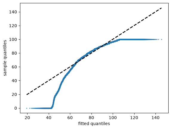
The points bend downwards, which is the mirror image of the house price figure.
At the left-hand end the sample quantiles fall well below the fitted ones, because the data have a long left tail of deaths at young ages that the normal distribution cannot reproduce.
The figure also shows a second, unrelated problem: the points run flat along \(y = 100\) at the right-hand end.
That is the “100 and over” category, which caps every age at 100.
A Q-Q plot displays such recording conventions very clearly, since they show up as flat segments where many observations share a single value.
Exercise 6.4
The next data set records the full-time score of every match in ten seasons of the English Premier League.
url = ('https://github.com/QuantEcon/data-lectures/raw/main/'
       'lectures/epl_match_goals.csv')
matches = pd.read_csv(url)
The Poisson distribution from Probability Distributions has one parameter \(\lambda\), and both its mean and its variance equal \(\lambda\).
Compute the total number of goals in each match and check whether its mean and variance are close.
Then fit a Poisson distribution by the method of moments and compare its probabilities with the observed frequencies.
Why might this model work well for goals?
Solution
The columns home_goals and away_goals hold the scores.
url = ('https://github.com/QuantEcon/data-lectures/raw/main/'
       'lectures/epl_match_goals.csv')
matches = pd.read_csv(url)
goals = matches['home_goals'] + matches['away_goals']
goals.mean(), goals.var()
(2.83, 2.7770939720979206)
These are close, which is encouraging.
u = scipy.stats.poisson(goals.mean())

counts = goals.value_counts().sort_index()
frequencies = counts / counts.sum()
S = np.arange(counts.index.max() + 1)

fig, ax = plt.subplots()
ax.bar(counts.index, frequencies, alpha=0.4, label='observed frequency')
ax.plot(S, u.pmf(S), linestyle='', marker='o', color='C1',
        label='fitted Poisson')
ax.vlines(S, 0, u.pmf(S), lw=0.5, color='C1')
ax.set_xlabel('goals per match')
ax.set_ylabel('probability')
ax.legend()
plt.show()
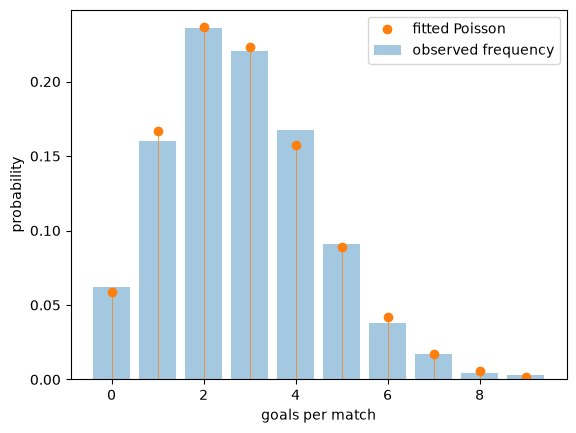
The fit is good.
Goals are rare events, arising at a roughly constant rate over the course of a match and largely independently of each other, which are exactly the conditions under which the Poisson distribution arises.
Exercise 6.5
The next data set records every earthquake of magnitude 5 and above in the region around Japan between 2000 and 2024, as reported by the US Geological Survey.
url = ('https://github.com/QuantEcon/data-lectures/raw/main/'
       'lectures/japan_earthquakes.csv')
quakes = pd.read_csv(url)
Earthquakes are often modeled as arriving randomly and independently at some constant rate.
If that is true, then the time between successive earthquakes is exponentially distributed.
Using these data, compute the time in days between successive earthquakes, fit an exponential distribution by the method of moments, and assess the fit.
(The exponential distribution has one parameter \(\lambda\) and mean \(1/\lambda\).)
Does the model hold up?
Solution
Here is one solution.
url = ('https://github.com/QuantEcon/data-lectures/raw/main/'
       'lectures/japan_earthquakes.csv')
quakes = pd.read_csv(url)

times = pd.to_datetime(quakes['time'], format='ISO8601')
gaps = times.diff().dropna().dt.total_seconds() / (60 * 60 * 24)

u = scipy.stats.expon(scale=gaps.mean())

fig, ax = plt.subplots()
qq_plot(gaps, u, ax)
plt.show()
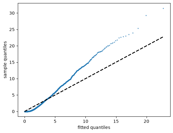
The fit fails badly, with the largest gaps far longer than the exponential distribution predicts.
A second diagnostic makes the problem clearer.
For the exponential distribution the standard deviation equals the mean.
gaps.mean(), gaps.std()
(2.5645754636399616, 3.765224536996305)
The standard deviation is around half again the mean, so the data are much more variable than the model allows.
The reason is that earthquakes are not independent.
Large earthquakes are followed by aftershocks, so events arrive in clusters, with long quiet periods in between.
This connects to our discussion of independence: a sample tells us about a distribution only when its observations bring new information, and an aftershock tells us mostly what the main shock already did.